
Start with the physical problem
Model selection is a process of matching assumptions, not ranking methods from best to worst. Geometry, boundary behavior, material contrast, acoustic size, and the desired scattering quantity all matter. A more elaborate formulation is not necessarily more appropriate for a poorly matched target (Clay and Horne 1994; Stanton 1996; Jech et al. 2015).
Before choosing a model, identify:
- the target’s gross geometry and any important internal components,
- the applicable boundary condition or material description,
- the frequency and orientation range,
- whether the target is weakly scattering, resonant, or acoustically large,
- whether the calculation requires monostatic backscatter, bistatic scattering, orientation averaging, or retained complex amplitude, and
- whether the proposed model is validated over the required scope.
The flowchart provides a first pass through those decisions. It narrows the candidate set but does not replace the assumptions and validation statements on each model’s pages:
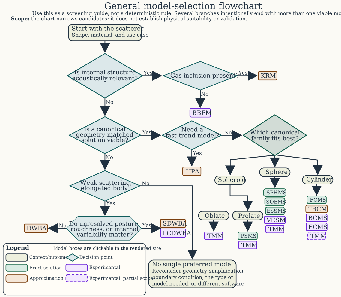
Select a model label to open that model family’s overview.
Choose the physical representation first
Canonical shapes
Canonical models are the natural starting point when a sphere, prolate spheroid, or finite cylinder is a defensible representation. Their coordinate systems follow the boundary closely and often permit exact or modal-series solutions (Morse and Feshbach 1953; Bowman et al. 1987). The boundary still has to match. A rigid sphere, a fluid sphere, an elastic shell, and a solid elastic calibration sphere share a shape but not the same interface physics.
| Target representation | Primary candidates | Main distinction |
|---|---|---|
| Homogeneous sphere | SPHMS, TMM | SPHMS directly solves the spherical modal problem. TMM is useful when retained transition-matrix products or angular post-processing are required. |
| Solid elastic calibration sphere | SOEMS | Includes longitudinal and shear waves in the solid. |
| Elastic spherical shell | ESSMS | Resolves shell elasticity and the interior fluid. |
| Prolate spheroid | PSMS, TMM | PSMS is the geometry-matched modal series. TMM supports a retained matrix workflow. |
| Finite circular cylinder | FCMS, TMM | FCMS is the direct finite-cylinder modal family. The documented TMM cylindrical scope is narrower. |
HPA can provide a faster asymptotic comparison for several smooth canonical shapes. It does not reproduce all boundary or resonance physics of the corresponding modal solution.
Arbitrary or segmented bodies
For weakly scattering elongated fluid-like bodies, DWBA is usually the first candidate. It integrates contributions along a body whose density and sound-speed contrasts remain sufficiently small. SDWBA uses the same general physical setting but introduces phase variability to represent unresolved roughness, posture, or other sources of incoherence (Stanton et al. 1998; Demer and Conti 2003). Use DWBA for a specified deterministic target state. Use SDWBA when the distribution of unresolved phase variation is part of the intended model.
PCDWBA is available for polynomially described cylindrical bodies. Its geometry and approximation assumptions should be checked against the PCDWBA theory page before treating it as a general replacement for DWBA.
For a fish-like target in which a gas-filled swimbladder is an explicit and important component, KRM is often the most natural first model. Its hybrid treatment is intended for the body-plus-swimbladder problem, not merely for any elongated outline (Clay 1992; Foote 1982).
BBFM represents a body assembled from boundary elements. It is relevant when explicit boundary geometry is more important than a canonical or centerline reduction. Review its current validation scope and computational cost before selecting it only because the geometry is complex.
Match the acoustic regime
Geometry alone does not identify the dominant scattering mechanism. Two models can accept similar shapes while describing different regimes:
- TRCM describes high-frequency, locally cylindrical scattering through coherent reflected and transmitted ray contributions.
- DWBA describes weak-contrast volume scattering.
- FCMS resolves finite-cylinder modal behavior.
- HPA retains broad high-frequency trends with fewer of the details present in a geometry-matched modal solution.
Acoustic size should therefore be considered together with contrast and boundary condition. A cylinder does not become a TRCM problem solely because it is cylindrical, and an elongated target does not become a DWBA problem if its contrast violates the weak-scattering premise.
Match the requested output
Most package models are organized around monostatic backscatter and reported target strength. That is not the only possible scattering calculation. The TMM family can retain transition-matrix information for bistatic scattering, angular grids, and orientation post-processing. Select a model that produces the quantity needed by the analysis rather than assuming a backscatter spectrum can answer every angular-scattering question (Mishchenko et al. 2002; Waterman 1971).
Output requirements can also affect whether complex amplitude must be retained. Target strength is suitable for logarithmic reporting. Coherent combination requires phase-bearing amplitude, while energetic averaging is performed in a linear cross-section domain. See Comparing models on the same target when the decision depends on how two defensible formulations differ.
When more than one model is defensible
Model overlap is expected. Useful comparisons include:
- DWBA and SDWBA to assess the effect of phase variability,
- FCMS and TRCM to compare modal and high-frequency ray descriptions,
- SPHMS or PSMS and HPA to assess the loss of detail in an asymptotic approximation, and
- a canonical model and TMM when retained angular products are required.
Keep geometry, material properties, medium properties, orientation, frequency, and output definition fixed during the comparison. A difference then reflects model structure more cleanly. If those inputs change at the same time, the exercise becomes a broader sensitivity study.
Check scope before committing to a model
A compatible object class only establishes that the software can dispatch the model. It does not establish physical suitability. Before using a result:
- read the model’s theory page and identify its boundary and approximation assumptions,
- read the implementation page for supported shapes, options, and numerical controls,
- inspect the model’s status in Validation and benchmark reproduction, and
- test sensitivity to the model choice when a neighboring formulation is also defensible.
The best initial model is the simplest one that retains the geometry, boundary physics, scattering configuration, and numerical fidelity required by the scientific question.