Building scatterers • acousticTS

Introduction

The scatterer classes in acousticTS are organized around target types that recur across fisheries and zooplankton acoustics, from calibration spheres to weakly scattering elongated bodies and composite fish targets.

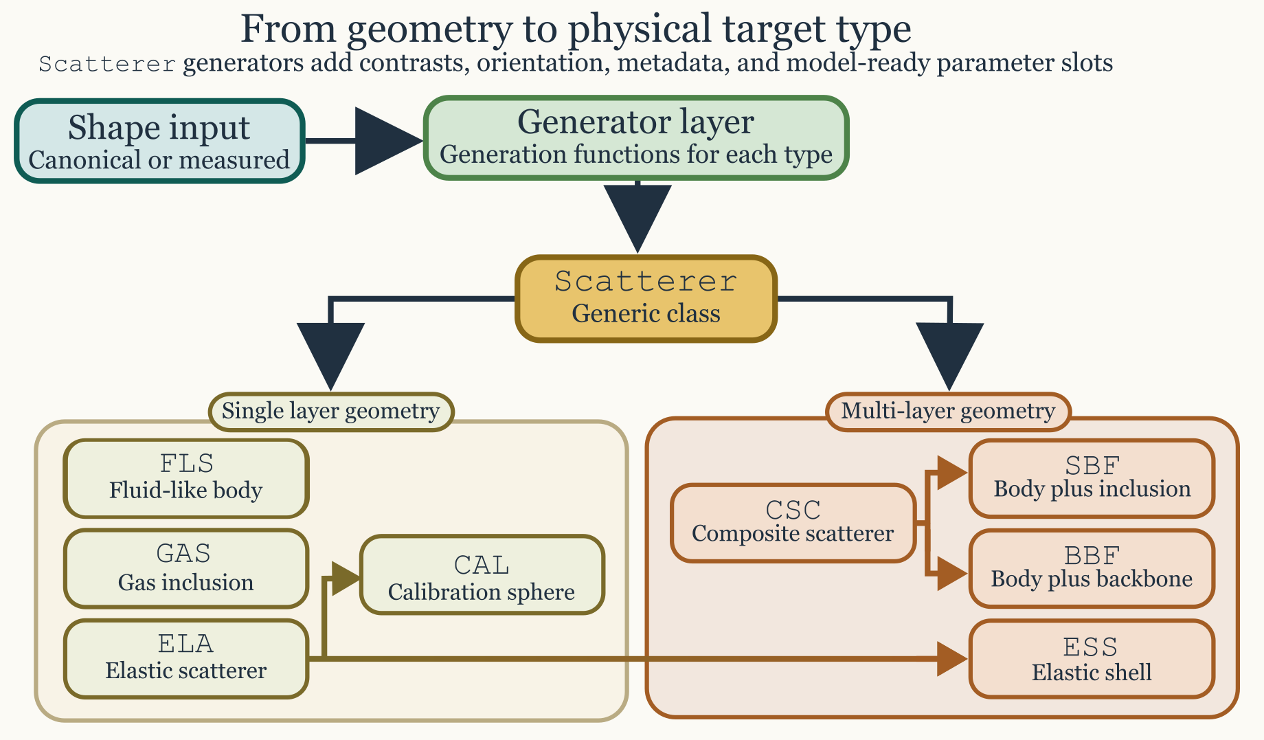
Once a geometry exists, it still has to be assigned a physical interpretation before most models in acousticTS can be run. That is the role of a scatterer object. A shape answers the geometric question, but a scatterer answers the acoustic one: what is the target made of, which interfaces matter, how should the surrounding medium be interpreted, and which class of model assumptions is meant to apply?

This distinction matters because the same outline can support several different physical interpretations. A smooth elongated body might be treated as a weakly scattering fluid-like target, as a gas-filled inclusion, or as part of a composite fish-like target with an internal swimbladder. The geometry by itself does not decide among those cases. Scatterer construction is the step where the reader turns a geometric description into a model-ready acoustic object.

Updated scatterer-generation and class-hierarchy map

Quick constructor examples

The fastest way to see the package logic is to build a few small objects directly.

library(acousticTS)

shape_obj <- prolate_spheroid(
  length_body = 0.04,
  radius_body = 0.004,
  n_segments = 60
)

fls_obj <- fls_generate(
  shape = shape_obj,
  density_body = 1045,
  sound_speed_body = 1520
)

gas_obj <- gas_generate(
  shape = sphere(radius_body = 0.01, n_segments = 60),
  g_fluid = 0.0012,
  h_fluid = 0.22
)

data.frame(
  object_class = c(class(fls_obj)[1], class(gas_obj)[1]),
  shape = c(
    extract(fls_obj, c("shape_parameters", "shape")),
    extract(gas_obj, c("shape_parameters", "shape"))
  ),
  length_m = c(
    extract(fls_obj, c("shape_parameters", "length")),
    extract(gas_obj, c("shape_parameters", "length"))
  )
)

##   object_class           shape length_m
## 1          FLS ProlateSpheroid     0.04
## 2          GAS          Sphere     0.02

That is the core pattern used throughout the package: build a Shape, then assign it a physical interpretation with the relevant scatterer constructor.

It is also worth checking the geometry visually at this stage because the scatterer plot reflects the stored object that will be passed into target_strength(), not just the constructor inputs.

old_par <- par(no.readonly = TRUE)
on.exit(par(old_par), add = TRUE)

par(mfrow = c(1, 2), mar = c(3, 3, 2.2, 0.8))
plot(fls_obj, type = "shape", main = "FLS object")
plot(gas_obj, type = "shape", main = "GAS object")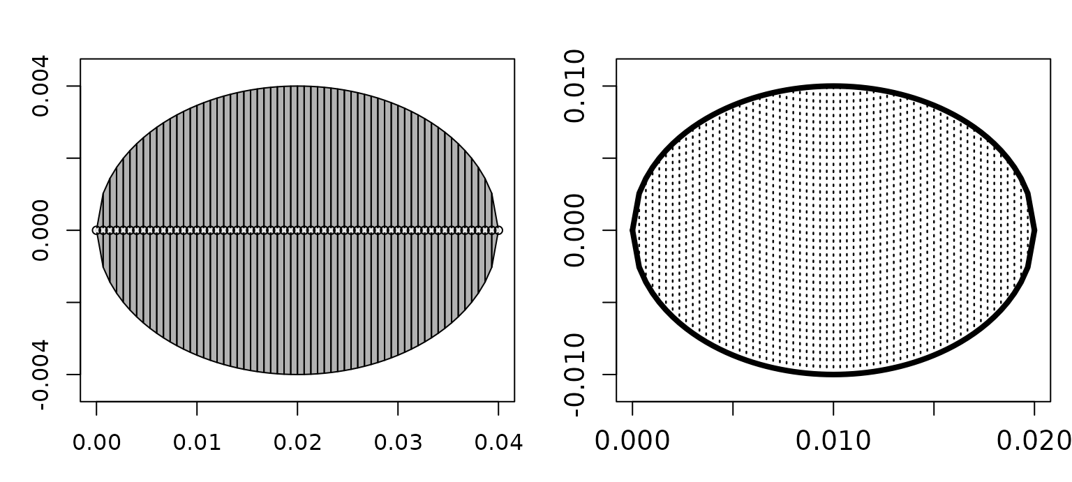

Why scatterer construction is separate from shape construction

The package separates shape generation from scatterer generation so that geometry can be reused across several physical scenarios. That separation is more than a software convenience. It mirrors the modeling logic used throughout the package. In acoustics, geometry and material contrast are related, but they are not the same thing. A user may want to ask how the same body behaves when interpreted as fluid-like rather than gas-filled, or how a measured outline behaves when modeled with a simple weak-scattering approximation versus a more specialized composite model.

Keeping those stages separate also reduces ambiguity. When the object is built in two steps, it becomes much easier to see whether a later disagreement comes from geometry, from material properties, or from model choice. That is one of the central design ideas behind the package.

Main generator families

The most important constructors are fls_generate() for fluid-like segmented bodies, gas_generate() for gas-filled simple bodies, sbf_generate() for fish-like body-plus-internal-structure targets, ess_generate() for elastic-shelled spheres, and cal_generate() for calibration spheres. Each constructor packages geometry, material properties, metadata, units, and model-ready parameter fields into a single scatterer object, but they do so for different acoustic interpretations.

fls_generate() is the general fluid-like constructor and is often the right starting point for weakly scattering elongated targets used with DWBA, SDWBA, HPA, TRCM, or other fluid-like workflows. gas_generate() is more specialized. It is intended for simple gas-filled objects where the dominant acoustic contrast comes from the gas-fluid interface. sbf_generate() is meant for composite fish-like targets where body and internal structures, especially a swimbladder, need to be represented together rather than collapsed into one homogeneous body. ess_generate() is reserved for elastic shelled spheres, where shell thickness and elastic material properties are central to the physics. cal_generate() is the constructor for standard calibration spheres, where the target is not a biological body at all but a well-defined solid sphere used for reference and validation work.

The practical consequence is that constructor choice should be driven by the interface physics that matter most, not only by the overall silhouette of the target.

The map above makes the class hierarchy explicit as well. Scatterer remains the common parent, but composite targets branch through CSC, elastic-target families branch through ELA, and the swimbladder-bearing and backbone-bearing composite targets are separated into SBF and BBF rather than being implied by one generic fish-only path. That makes the difference between generator choice and class inheritance much more transparent.

Recommended constructor convention

The clearest workflow is:

Build geometry with a Shape constructor.
Pass that geometry into the relevant scatterer constructor.
Supply material properties either as contrasts or as absolute values.

In practice, that means the public convention is:

single-component targets: shape = <Shape>
composite targets: body_shape = <Shape>, bladder_shape = <Shape>, or backbone_shape = <Shape>

For example, a fluid-like target should usually be built with a call like fls_generate(shape = my_shape, ...), not by asking fls_generate() to also invent the geometry internally. Likewise, sbf_generate() is clearest when the body and swimbladder are built separately and passed in explicitly as body_shape and bladder_shape.

Older entry points remain available for compatibility, but they should be treated as compatibility-only rather than preferred public interfaces. Raw coordinate vectors remain a supported manual geometry pathway. Character shape labels such as "sphere" or "arbitrary" are still accepted so that older scripts continue to run, but that string-dispatch pattern is deprecated. Internally, every accepted pathway is normalized to the same Shape-first geometry contract as the explicit workflow.

The same simplification applies to units. Scatterer constructors are standardized to meters for geometry and radians for orientation. Compatibility arguments like length_units, radius_units, diameter_units, and theta_units are accepted so that older calls do not fail abruptly, but non-SI values are deprecated compatibility inputs rather than an encouraged part of the public workflow.

Material inputs remain flexible by design. For each component, density and sound speed may be supplied either as contrasts (g_*, h_*) or as absolute properties (density_*, sound_speed_*). That flexibility is useful and does not add the same kind of cognitive overhead as overloading the geometry interface.

body_shape <- arbitrary(
  x_body = c(0, 0.08, 0.12),
  zU_body = c(0.001, 0.004, 0.001),
  zL_body = c(-0.001, -0.004, -0.001)
)

bladder_shape <- arbitrary(
  x_bladder = c(0.03, 0.08, 0.1),
  zU_bladder = c(0.0008, 0.0016, 0.0008),
  zL_bladder = c(-0.0008, -0.0016, -0.0008)
)

sbf_obj <- sbf_generate(
  body_shape = body_shape,
  bladder_shape = bladder_shape,
  density_body = 1040,
  sound_speed_body = 1500,
  density_bladder = 1.2,
  sound_speed_bladder = 340
)

data.frame(
  body_length_m = extract(sbf_obj, c("shape_parameters", "body", "length")),
  bladder_length_m = extract(sbf_obj, c("shape_parameters", "bladder", "length")),
  body_theta_rad = extract(sbf_obj, c("body", "theta"))
)

##   body_length_m bladder_length_m body_theta_rad
## 1          0.12             0.07       1.570796

That is the composite pattern: build the components separately, then hand them to the scatterer generator explicitly as body_shape, bladder_shape, or backbone_shape.

At that point it is often useful to inspect the object internals directly so the separation between components is explicit in code as well as in the plot.

list(
  body_length_m = extract(sbf_obj, c("shape_parameters", "body", "length")),
  bladder_length_m = extract(sbf_obj, c("shape_parameters", "bladder", "length")),
  body_theta_rad = extract(sbf_obj, c("body", "theta")),
  bladder_x_head = head(extract(sbf_obj, "bladder")$rpos[1, ])
)

## $body_length_m
## [1] 0.12
## 
## $bladder_length_m
## [1] 0.07
## 
## $body_theta_rad
## [1] 1.570796
## 
## $bladder_x_head
## [1] 0.03 0.08 0.10

Matching class to target type

The scatterer class should match the intended physical interpretation, not just the geometry. For example, a smooth elongated body may be represented geometrically by a prolate spheroid, but its scatterer class still depends on whether it is being treated as fluid-like, gas-filled, or composite. That distinction is the reason the decision guide branches from a single geometric starting point into several different scatterer families. The package is asking not only what the target looks like, but also which material interfaces and internal components are meant to matter acoustically.

This is where many avoidable workflow errors begin. A target can have a reasonable geometric representation and still be assigned to the wrong scatterer class. When that happens, the later model run may appear to fail even though the real problem is that the object was given the wrong physical meaning. For that reason, it is often worth pausing at the scatterer-construction stage and checking whether the object class truly matches the intended boundary interpretation and internal structure.

Common parameter groups

Most scatterer generators require some combination of geometry or a pre-built Shape, density and sound-speed information or their contrasts, orientation, unit declarations, and optional metadata identifiers. That recurring structure is intentional. It means that once a scatterer has been built correctly, the same object can later be passed through one or several compatible models without rebuilding it from scratch.

One of the most important practical decisions at this stage is whether to parameterize the object with absolute properties or with contrasts. In many workflows the package can derive contrasts internally when only absolute density and sound speed are supplied, which is convenient when the underlying data come from direct measurements or literature tables. In other workflows, the scientifically natural description is already contrast-based, especially for weakly scattering or gas-filled approximations. The important point is not that one representation is always better, but that the chosen representation should remain physically consistent with the surrounding medium and with the intended model assumptions.

Orientation and units matter here as well. Scatterer construction is often where body angle, segment spacing, diameter units, and other bookkeeping fields first become fixed. If those are wrong at this stage, the later model output may look implausible for reasons that have nothing to do with the mathematics of the model itself.

A practical way to think about the constructors

One useful mental model is that scatterer constructors define the acoustic identity of the object. If the question is about a weakly contrasting body, start from the fluid-like constructor. If the dominant physics is a gas interface, use the gas-filled constructor. If the target is explicitly composite, use the constructor that keeps those components separate. If the target is a canonical shell or a calibration sphere, use the constructor written for that specific physics rather than forcing the object into a more generic class.

That approach keeps the workflow honest. It also makes later model selection much easier, because compatible model families become apparent as soon as the scatterer class is chosen. In that sense, good scatterer construction is already the beginning of good model selection.

The same shape-first pattern extends to the other target families as well:

# Explicit body-plus-backbone target for BBFM workflows
bbf_obj <- bbf_generate(
  body_shape = arbitrary(
    x_body = c(0, 0.04, 0.08),
    zU_body = c(0.001, 0.004, 0.001),
    zL_body = c(-0.001, -0.004, -0.001)
  ),
  backbone_shape = cylinder(
    length_body = 0.05,
    radius_body = 0.0008,
    n_segments = 40
  ),
  density_body = 1070,
  sound_speed_body = 1570,
  density_backbone = 1900,
  sound_speed_longitudinal_backbone = 3500,
  sound_speed_transversal_backbone = 1700
)

# Standard calibration sphere
cal_obj <- cal_generate(
  material = "WC",
  diameter = 38.1e-3,
  n_segments = 120
)

# Elastic-shelled sphere
ess_obj <- ess_generate(
  shape = sphere(radius_body = 0.03, n_segments = 80),
  shell_thickness = 0.001,
  density_shell = 1050,
  sound_speed_shell = 2350,
  density_fluid = 1030,
  sound_speed_fluid = 1500,
  E = 3.5e9,
  nu = 0.34
)

cal_obj <- cal_generate(
  material = "WC",
  diameter = 38.1e-3,
  n_segments = 120
)

ess_obj <- ess_generate(
  shape = sphere(radius_body = 0.03, n_segments = 80),
  shell_thickness = 0.001,
  density_shell = 1050,
  sound_speed_shell = 2350,
  density_fluid = 1030,
  sound_speed_fluid = 1500,
  E = 3.5e9,
  nu = 0.34
)

data.frame(
  object_class = c(class(cal_obj)[1], class(ess_obj)[1]),
  diameter_m = c(
    extract(cal_obj, c("shape_parameters", "diameter")),
    NA_real_
  ),
  shell_thickness_m = c(
    NA_real_,
    extract(ess_obj, c("shell", "shell_thickness"))
  )
)

##   object_class diameter_m shell_thickness_m
## 1          CAL     0.0381                NA
## 2          ESS         NA             0.001

What to check before moving on

Before running a model, it is worth checking a few simple things. The geometry should be the one you intended to build. The scatterer class should match the physical target type rather than just the body outline. Material properties or contrasts should be internally consistent. Orientation and units should be explicit. If the target is composite, the components that matter acoustically should still be represented separately rather than accidentally collapsed into one homogeneous body.

Those checks are simple, but they have a large payoff. Many apparent modeling problems are actually scatterer-construction problems discovered too late.

extract(fls_obj, c("body", "density"))

## [1] 1045

extract(fls_obj, c("shape_parameters", "shape"))

## [1] "ProlateSpheroid"

That kind of quick inspection is usually enough to confirm that the object you built matches the target type you intended before moving on to target_strength().

Recommended next step

After building a scatterer, the next action is usually to run a compatible model and inspect TS, sigma_bs, or any stored intermediate outputs needed for interpretation. The practical continuation of this article is running target strength models, while the conceptual continuation is choosing a model.