Package concepts

Introduction

The package concepts reflect the same divide between exact solutions, asymptotic approximations, and organism-specific composites seen in the scattering literature (jech_etal_2015?; stanton_acoustic_1996?).

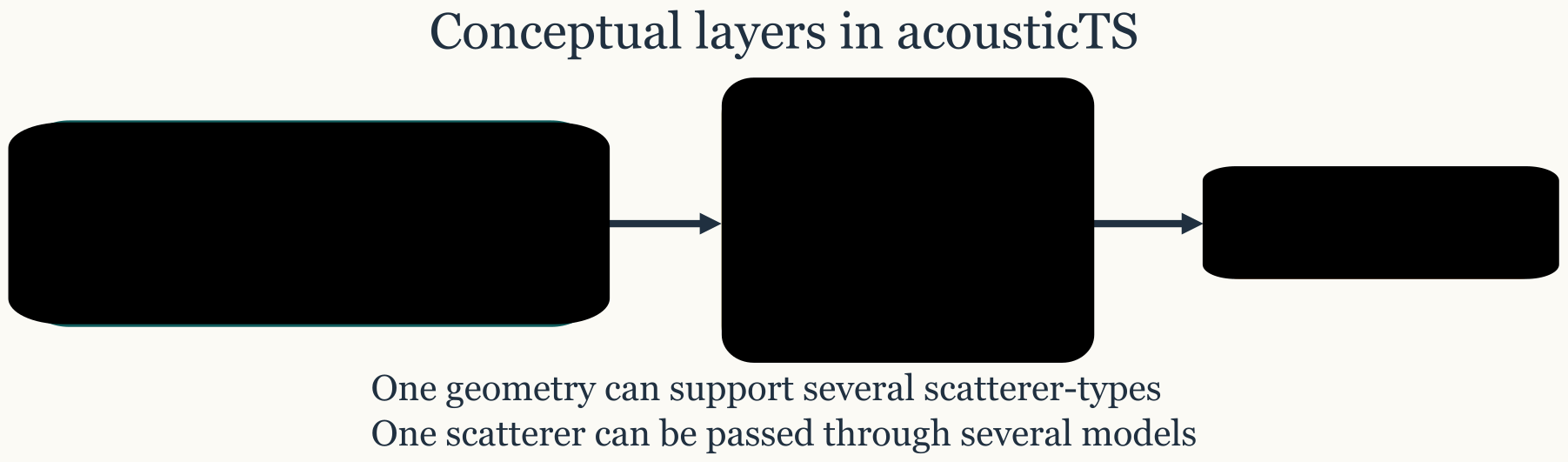
The package is easiest to use once three ideas are kept separate: geometry, physical target type, and scattering model. Those three ideas are related, but they are not interchangeable. Many practical mistakes in acousticTS come from confusing one of those layers with another, such as treating a shape as if it were already a physical scatterer, or treating a model name as if it defined the target itself.

This page is the conceptual map for the rest of the documentation. The goal is not to derive any model. The goal is to stabilize the package vocabulary before moving into theory pages and workflow pages. If readers understand why the package separates geometry from scatterer meaning and scatterer meaning from model choice, most of the later documentation becomes much easier to navigate.

Shapes versus scatterers

A Shape describes geometry only. It answers geometric questions such as whether the target is spherical, cylindrical, prolate spheroidal, or arbitrary, and it stores the coordinate or discretization information needed to represent that geometry. A shape by itself does not say whether the target is fluid-like, gas-filled, shelled, elastic, or calibration-like. It is only the geometric scaffold.

A Scatterer object adds physical interpretation to that scaffold. It says what the target is made of, which components are present, how the body is oriented, and what material contrasts or elastic quantities should later be passed to a scattering model. This is the stage at which a geometric outline becomes an acoustically meaningful target.

The distinction matters because the same geometry can appear in more than one physical regime. A sphere-shaped geometry may be used as a gas-filled sphere in SPHMS, a fluid sphere in HPA, an elastic-shelled sphere in ESSMS, or a calibration sphere in the calibration workflow. In all four cases the outer geometry may still be spherical. What changes is the physical interpretation of the boundary and material properties. The package keeps that distinction explicit because it makes model choice, debugging, and comparison much more transparent.

This is one of the most important conceptual decisions in the package. Geometry answers “what does the target look like?” A scatterer answers “what kind of thing is it physically?” Those questions overlap, but they are not identical. A shape can be reused across several scatterer classes, and a scatterer class can sometimes be applied to several shapes. The package design keeps that flexibility visible rather than hiding it inside a single overloaded constructor.

Scatterer classes

The package uses several high-level scatterer classes, including FLS for fluid-like scatterers, GAS for gas-filled simple bodies, SBF for swimbladder-bearing fish-like targets, ESS for elastic-shelled spheres, and CAL for calibration spheres. These classes are not just labels. They determine which physical components the object should carry and which model families are naturally compatible with that target description.

In practical terms, class selection answers the question, “What kind of information should this object contain?” An FLS object is the natural starting point for weakly scattering fluid-like bodies. A GAS object is appropriate when the relevant physics is dominated by a gaseous or highly compressible inclusion. An SBF object is built for workflows where a body and swimbladder need to remain distinct. An ESS object is for shell problems where the shell material and the internal fluid both matter. A CAL object is for calibration targets where the material definition is intentionally more constrained.

Those classes also determine the internal component structure of the object. An FLS object carries a body slot. An SBF object carries body and bladder. An ESS object carries shell and fluid. That organization is what lets the package reuse generic functions such as plot() and extract() across very different kinds of targets without collapsing them into one indistinct object type.

This is also why class choice is a conceptual decision rather than a purely technical one. Choosing a class says what components the package should expect the target to have and what kinds of model assumptions can later be attached to it cleanly. When the wrong class is chosen, the problem is not only that a later function call becomes awkward. It is that the package has been asked to represent the wrong kind of target from the start.

Object structure in practice

Almost every scatterer object is organized around the same broad layers of information. There is metadata for IDs and bookkeeping, shape_parameters for geometric metadata, one or more physical component slots such as body, bladder, shell, or fluid, a model_parameters slot for the intermediate parameterization a specific model needs, and a model slot for the final outputs. The exact details differ by class, but the logic is stable across the package.

That arrangement is easiest to see with a small example.

library(acousticTS)

shape_obj <- cylinder(
  length_body = 0.03,
  radius_body = 0.0025,
  n_segments = 60
)

scatterer_obj <- fls_generate(
  shape = shape_obj,
  density_body = 1045,
  sound_speed_body = 1520,
  theta_body = pi / 2,
  ID = "example-cylinder"
)

names(scatterer_obj@metadata)

## [1] "ID"

names(scatterer_obj@body)

## [1] "rpos"                   "radius"                 "theta"                 
## [4] "g"                      "h"                      "density"               
## [7] "sound_speed"            "radius_curvature_ratio"

names(scatterer_obj@shape_parameters)

## [1] "length"                 "radius"                 "n_segments"            
## [4] "radius_curvature_ratio" "taper_order"            "shape"                 
## [7] "length_units"           "theta_units"

At this point the object is physically defined, but no target-strength model has been run yet. That is why model_parameters and model begin as empty containers and are populated only after target_strength() is called. This delayed population is a useful design choice. It means the target object can exist first as a stable physical description, and only later acquire model-specific parameterizations and predictions.

That separation is valuable because it keeps debugging ordered. Readers can inspect the geometry, inspect the physical parameters, and verify the target representation before they ever ask the package to predict backscatter. Once model output is attached, the full object still carries the original geometry and physical meaning with it, which makes later comparison and validation much easier.

Models as separate layers

Models in acousticTS are not the same thing as scatterers. A model is a mathematical mapping from the scatterer description and acoustic conditions to predicted backscatter. This is why the package can support multiple models for the same target. A fluid-like elongated object might be explored with DWBA, SDWBA, TRCM, HPA, or another more canonical model depending on the question being asked and the approximation regime that is defensible.

This separation is one of the most useful design choices in the package because it means you do not have to rebuild the target every time you ask a different modeling question. One object can support several model runs, provided the geometry and physical interpretation are compatible with those models.

frequency <- seq(38e3, 120e3, by = 6e3)

scatterer_obj <- target_strength(
  object = scatterer_obj,
  frequency = frequency,
  model = c("dwba", "hpa")
)

names(extract(scatterer_obj, "model"))

## [1] "DWBA" "HPA"

At the conceptual level, the important point is that a model is a lens applied to the same physical target, not a replacement for the target object itself. That way of thinking is especially helpful when several models are reasonable. Readers do not need to decide that one object is a DWBA object and another is an HPA object. Instead, they can define one physically meaningful target and then ask what different model families predict for it.

This keeps model comparison tied to a common target description instead of letting the object definition drift from one comparison to the next. The choosing a model article is the practical guide to that decision, while the model theory pages explain the mathematical tradeoffs in detail.

Stored results and traceability

Model outputs are written back onto the scatterer object rather than returned as entirely unrelated standalone structures. This makes it easier to compare multiple models on the same target, retain geometry and parameter metadata, plot shape and model output from the same object, and inspect nested results with extract().

That becomes especially useful when comparison is the real goal. A user can keep one object in memory, run several models, and then pull the corresponding sub-results by name.

head(extract(scatterer_obj, "model")$DWBA)

##   frequency        ka                        f_bs     sigma_bs        TS
## 1     38000 0.3979351 -6.723778e-05-1.940150e-20i 4.520919e-09 -83.44773
## 2     44000 0.4607669 -8.773690e-05-2.931388e-20i 7.697764e-09 -81.13635
## 3     50000 0.5235988 -1.097965e-04-4.168663e-20i 1.205527e-08 -79.18823
## 4     56000 0.5864306 -1.328846e-04-5.650686e-20i 1.765833e-08 -77.53050
## 5     62000 0.6492625 -1.564363e-04-7.364911e-20i 2.447231e-08 -76.11325
## 6     68000 0.7120943 -1.798640e-04-9.287346e-20i 3.235107e-08 -74.90111

head(extract(scatterer_obj, "model")$HPA)

##   frequency     sigma_bs        TS
## 1     38000 3.087454e-09 -85.10400
## 2     44000 4.476195e-09 -83.49091
## 3     50000 5.951762e-09 -82.25354
## 4     56000 7.447037e-09 -81.28017
## 5     62000 8.924453e-09 -80.49418
## 6     68000 1.036723e-08 -79.84337

The practical advantage is traceability. When the result stays attached to the same object that carries geometry, material properties, and metadata, it is much easier to see which assumptions generated which curve. This reduces one of the most common sources of confusion in modeling workflows, namely losing track of which result belongs to which target parameterization.

It is also the reason the package can support workflow pages such as comparison, simulation, and validation without requiring a separate results-management system. The object itself becomes the local record of what was modeled, under what assumptions, and with what outcome.

A practical mental model

For most workflows, the simplest mental model is the following. A Shape answers “what is the geometry?” A Scatterer answers “what kind of target is this physically?” target_strength() answers “which model should be applied under which acoustic conditions?” extract() and plot() answer “what came out, and how do I inspect it?”

That mental model is enough to keep most workflows organized even before the theory pages come into play. It also suggests a useful debugging order. If a result looks wrong, first ask whether the geometry is right. Then ask whether the scatterer class and material meaning are right. Only then ask whether the chosen model is the right one, or whether its numerical settings need adjustment. That order usually isolates problems faster than jumping directly to model equations.

Why this design is useful

This object separation allows the package to support both canonical theory and more empirical or workflow-oriented use cases. A user can build one target description and then ask several different questions of it without rebuilding the object from scratch each time. That is especially valuable in comparison studies, validation work, and exploratory parameter sweeps where consistency of target definition matters just as much as the model formulas themselves.

It also makes bookkeeping errors easier to catch. When geometry, material properties, and model outputs all remain attached to the same object, it is harder to lose track of which assumptions produced which target-strength curve. More broadly, this design lets the documentation stay modular without becoming fragmented. Workflow pages can focus on how to move through the package. Theory pages can focus on model assumptions. Concept pages like this one can focus on object meaning and package structure. Because the same object logic runs underneath all of them, those different kinds of documentation still connect cleanly.