Getting started with acousticTS

Introduction

The package workflow is meant to help users move between the same geometry, material, and model-choice questions that structure the broader fisheries-acoustics literature (jech_etal_2015?; stanton_acoustic_1996?; medwin_fundamentals_1998?).

This documentation is meant to be the first practical stop for readers who are new to acousticTS. The package covers several different target-strength models, several target classes, and several ways of building geometry, so the documentation can look broad at first glance. The easiest way to make that structure manageable is to keep one idea in mind from the beginning: the package separates geometry, physical interpretation, model choice, and result inspection on purpose. Those are related decisions, but they are not the same decision.

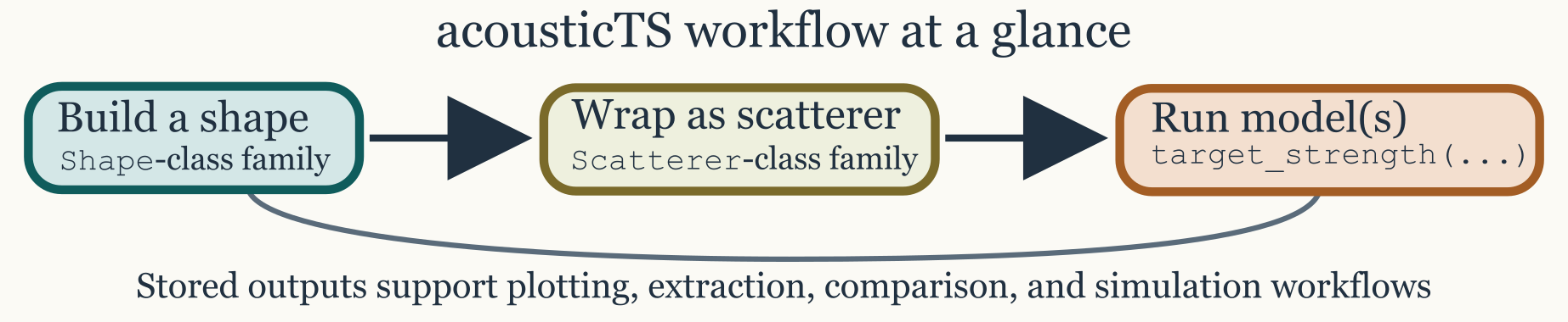
At the broadest level, every workflow moves through four layers. A Shape describes geometry only. A Scatterer object adds material properties, boundary interpretation, and metadata. A model call computes the backscattering response across a chosen frequency or acoustic-size range. Inspection and plotting then make it possible to decide whether the result is physically sensible before moving on to comparison, validation, or larger parameter sweeps. New users usually find the package much easier to navigate once those layers are kept conceptually separate.

This page does not attempt to replace the theory articles. Instead, it shows the workflow logic that links the rest of the documentation together. Readers should come away knowing what kinds of objects they will create, what choices they will need to make, and which later vignette to read when a particular decision becomes more detailed.

You can interact with certain figures by clicking diagram elements.

Quick example

The following example shows a compact but realistic package workflow. It builds a spherical gas-filled target, evaluates the spherical modal-series model, and then inspects the stored result. The same sequence of steps reappears across the rest of the package even when the geometry and model family change. What changes from vignette to vignette is usually not the overall workflow, but the physical meaning of the geometry and the assumptions built into the selected model.

library(acousticTS)

# 1. Create a geometry
sphere_shape <- sphere(radius_body = 0.05)

# 2. Create a scatterer by attaching acoustic contrasts
gas_sphere <- gas_generate(
  shape = sphere_shape,
  g_fluid = 0.0012,
  h_fluid = 0.22
)

# 3. Run a model
frequency <- seq(38e3, 120e3, by = 2e3)

gas_sphere <- target_strength(
  object = gas_sphere,
  frequency = frequency,
  model = "sphms",
  boundary = "gas_filled"
)

# 4. Inspect or plot
names(extract(gas_sphere, "model"))
plot(gas_sphere, type = "model")

This short example already contains the main package logic. The geometry is created first, because the model cannot be interpreted until the target shape is defined. Acoustic meaning is added second, because a sphere can represent very different physical targets depending on whether it is treated as gas-filled, fluid-filled, elastic, or something else entirely. The model is evaluated only after those assumptions are fixed. Inspection comes last, because even a successful model run still needs to be checked for physical plausibility.

In practice, most workflows differ only in the scatterer constructor and the model-specific arguments. A fluid-like elongated body may use fls_generate() and DWBA, a shell problem may use ess_generate() and ESSMS, and a calibration sphere may use cal_generate() and the calibration model. The package structure stays the same even when the acoustics do not. That consistency is deliberate. It allows readers to learn one workflow pattern and then reuse it across different geometries and model families.

The recommended pattern is to build geometry first and then hand that geometry to the scatterer constructor. In other words, sphere(), cylinder(), prolate_spheroid(), and arbitrary() answer the geometric question, while fls_generate(), gas_generate(), sbf_generate(), bbf_generate(), and ess_generate() answer the physical one. The supported public geometry pathways are therefore either a pre-built Shape object or explicit coordinate vectors supplied directly to the constructor. Older shorthand pathways based on character shape labels are compatibility-only and deprecated, so the shape-first workflow is the clearest one to learn and the least ambiguous one to debug.

Core concepts and objects

Understanding three core concepts makes the rest of the documentation much easier to navigate. A Shape is geometry only, whether that geometry is canonical, segmented, or imported from measured coordinates. A scatterer object is the physically interpreted target, meaning that it combines geometry with contrasts, densities, sound speeds, elastic properties, orientations, and any additional metadata needed by the model layer. Model results are then stored back onto that same object, typically as TS, sigma_bs, complex amplitudes, and model-specific bookkeeping fields.

The most common shape builders are sphere(), cylinder(), prolate_spheroid(), and arbitrary(). The most common scatterer constructors are fls_generate(), sbf_generate(), bbf_generate(), gas_generate(), ess_generate(), and cal_generate(). These answer two different questions. Shape builders answer “what is the geometry?” Scatterer constructors answer “what is the target physically?” That distinction matters because the same geometry may support several different physical interpretations, while the same physical interpretation may sometimes be explored over several different geometries.

It also helps to think of the package objects as progressively more informative descriptions of the same target. A shape alone is only a geometric scaffold. A scatterer object is the first stage at which the target becomes acoustically meaningful. A modeled object is then a target together with the consequences of a specific modeling assumption. Keeping those layers conceptually separate makes it easier to diagnose problems. If something looks wrong, the mistake may be geometric, physical, numerical, or interpretive, and those are best checked in that order.

Typical workflow

A robust first workflow usually begins with the simplest defensible representation of the target. If the target is close to a canonical shape, it is often helpful to start there because canonical geometry makes both interpretation and debugging easier. If the target is not well represented by a canonical body, an imported or segmented geometry may be more defensible. In either case, the goal is not to maximize geometric detail for its own sake. The goal is to choose a geometry that matches the model assumptions closely enough for the scientific question being asked.

Once the geometry is chosen, the next decision is the scatterer class. That choice should reflect the important material interfaces in the problem, not just the outline of the body. A fluid-filled body, a gas-bearing target, a shelled target, and a calibration sphere may all be smooth closed geometries, but they are not physically interchangeable. Much of the package structure is designed to keep that distinction explicit rather than implicit.

Only after the scatterer is physically defined does model choice become meaningful. At that stage, the main question is whether a geometry-matched exact or modal-series model exists, or whether an approximation better matches the target and the scientific objective. Frequency sweeps and orientation sweeps are then useful not only for producing figures, but also for deciding whether the response behaves plausibly before a larger batch run is attempted. A short exploratory run is often the best way to catch mismatched units, unrealistic material properties, or a model choice that does not fit the intended regime.

One of the most effective habits for new users is to inspect intermediate outputs early. Shape plots reveal geometry and orientation mistakes quickly. Stored model outputs reveal whether the requested model was attached and whether the expected quantities were produced. That small amount of checking usually saves more time than it costs, especially before a large sweep or comparison study.

Site map and documentation layout

The pkgdown site groups material into four layers to support different reading goals. Workflow articles like this one explain how to move through the package in practice. Conceptual articles explain why objects and workflows are organized the way they are. Theory pages document the mathematical assumptions and limits of each model family. Reference pages document the individual functions and data objects.

The most effective reading path for a new user is usually to begin with a workflow article, move to the companion conceptual page when object structure is unclear, and then use the theory pages to verify that the model choice is physically defensible. That order keeps the package approachable without collapsing the modeling assumptions into a single oversimplified tutorial.

Readers who already know the acoustics but are new to the package often take the opposite path: they begin with the theory page for the model they care about, then return to the workflow and object-building pages to see how those assumptions are encoded in practice. The documentation is meant to support both directions. The important point is that the package is easiest to use when geometry, physical interpretation, and model assumptions are treated as distinct but connected parts of the same workflow.

Introduction

Quick example

Core concepts and objects

Typical workflow

What to read next

Site map and documentation layout