Material Properties and Acoustic Utilities

Introduction

The property conventions on this page follow standard acoustics and elastic-wave references used throughout underwater scattering theory (Medwin and Clay 1998; Achenbach 1973).

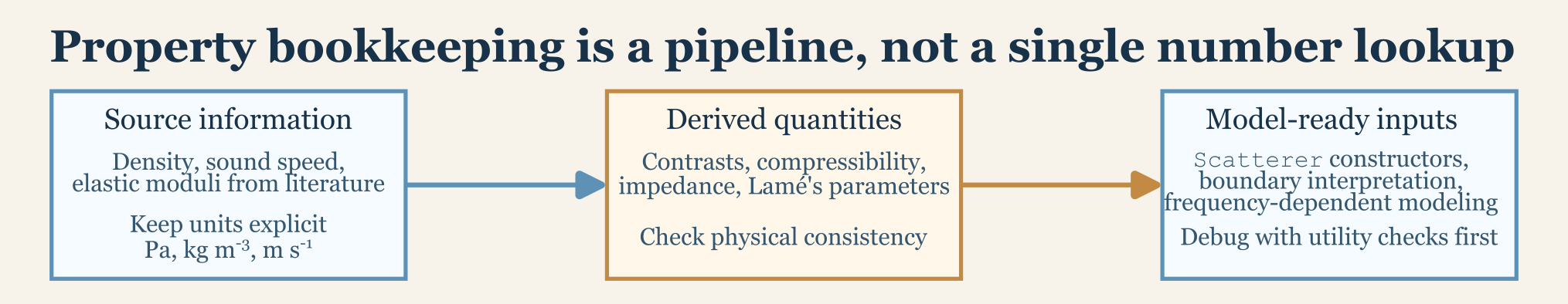
Many modeling errors are not caused by the scattering model itself. They are caused by incorrect material properties, inconsistent contrasts, or unit conversion mistakes. This article collects the supporting acoustic-property functions that feed the model layer and explains how to think about them physically before they are ever passed into a target-strength model.

In practice, this page is the bookkeeping companion to the theory pages. If a model result looks suspicious, one of the first things to check is whether the object was parameterized with sensible densities, sound speeds, contrasts, elastic constants, and medium properties. That may sound secondary compared with model choice, but it often is not. A theoretically appropriate model will still give an inappropriate answer if the target and medium properties do not describe the same physical situation the reader believes they are describing.

Main utility groups

The package includes utilities for density- and sound-speed-derived quantities, compressibility- and impedance-related calculations, elastic moduli such as Lamé parameters, shear modulus, Poisson ratio, and Young’s modulus, wavenumber and acoustic-size conversions, and logarithmic and linear-scale conversions. The functions are small, but they are central. Nearly every model in the package uses some subset of them, either explicitly or as part of the physical quantities from which the model inputs are built.

It is useful to think of these utilities as belonging to three different tasks:

1. converting between alternative descriptions of the same material,
2. checking whether target and medium contrasts are physically plausible, and
3. converting between reporting scales so that the model output is interpreted in the right domain.

That separation matters because a workflow can fail at any of those stages. A user may know the correct material but express it in the wrong parameterization. A user may compute a mathematically valid contrast that still does not correspond to the intended target. Or a user may obtain a correct model result and then summarize it in a domain that answers a different question.

Contrasts versus absolute properties

One of the most useful design choices in acousticTS is that many constructors and models accept either contrasts or absolute properties. A density contrast such as g_body expresses target density relative to the surrounding medium, while a sound-speed contrast such as h_body expresses target sound speed relative to the surrounding medium. Absolute properties such as density_body and sound_speed_body can often be supplied instead, with contrasts derived internally.

This flexibility is convenient, but it also means a user should be deliberate about which representation is being supplied. The package can often derive missing pieces, but it cannot rescue physically inconsistent inputs. If absolute properties imply one contrast and the manually supplied contrast implies another, the inconsistency belongs to the setup rather than to the scattering model.

The choice between contrasts and absolute properties is not only a coding convenience. It changes how the physical problem is being framed. Contrasts emphasize the target relative to the surrounding medium and are often the most natural way to think about weak-scattering approximations. Absolute properties emphasize the target itself and are often the most natural form when drawing from laboratory measurements or literature tables. Both are useful, but they should not be mixed casually.

It is also important to remember that a contrast is meaningless without an explicit reference medium. A value such as g_body = 1.02 says very little by itself unless the medium density is also understood. If the surrounding water properties change, the same absolute target properties imply different contrasts. That is one reason medium bookkeeping should remain visible in the workflow rather than being treated as an afterthought.

Acoustic utilities

Wavenumber

The acoustic wavenumber appears everywhere because it connects frequency and sound speed to acoustic size.

library(acousticTS)

frequency <- c(38e3, 70e3, 120e3)
sound_speed_sw <- 1500

wavenumber(frequency, sound_speed_sw)

## [1] 159.1740 293.2153 502.6548

That quantity underlies ka, reduced frequency, and many truncation rules. It is one of the simplest examples of why material bookkeeping matters. Changing only sound speed, while keeping the same nominal frequency and geometry, changes acoustic size and therefore changes which asymptotic or modal regime a model may be operating in.

This is also why frequency and sound speed should be checked together rather than separately. A frequency sequence may look reasonable on paper, but if the wrong sound speed is being used the implied acoustic-size range may not match the intended problem at all.

Linear and logarithmic conversion

Model outputs are often easier to compare in different domains depending on the question.

linear(-60)

## [1] 1e-06

db(1e-6)

## [1] -60

The practical rule is simple. Use TS in dB for reporting and communication, and use linear quantities such as sigma_bs when averaging, combining, or checking interference logic. Many avoidable interpretation errors arise from mixing those two roles.

This distinction matters well beyond plotting. If readers compare two models with RMSE, MAD, or other residual summaries, they should decide first whether the scientific question lives in the linear scattering domain or in the logarithmic reporting domain. A small dB discrepancy can correspond to a substantial difference in linear cross-section, and the reverse can also happen.

Compressibility contrast

The package also exposes simple interface-level calculations that are useful for sanity checks.

medium <- data.frame(density = 1026, sound_speed = 1500)
target <- data.frame(density = 1045, sound_speed = 1520)

compressibility(medium, target)

## [1] -0.04384916

Those utilities are especially helpful when a user wants to understand why a weak-scattering approximation is or is not plausible for a given target. Density contrast alone is rarely the whole story. Compressibility, impedance mismatch, and the joint behavior of density and sound speed are often the quantities that determine whether a target behaves as weakly scattering, strongly reflecting, or something in between (Medwin and Clay 1998).

This is one of the most common places where intuition can go wrong. A target may have density close to water but still differ noticeably in sound speed, or vice versa. Looking only at one property can therefore suggest a weak contrast when the combined interface behavior is more consequential.

Elastic utilities

Shell and solid-sphere models need elastic constants that are often reported inconsistently across sources. One paper may give E and \nu, another may give K and G, and a third may effectively imply Lamé parameters. The package utilities make it easier to move among those descriptions.

Representative functions include pois() for Poisson ratio, bulk() for bulk modulus, young() for Young’s modulus, shear() for shear modulus, and lame() for the Lamé parameter (Achenbach 1973).

E <- 7e10
nu <- 0.32

G <- shear(E = E, nu = nu)
K <- bulk(E = E, nu = nu)
lambda <- lame(E = E, nu = nu)

G

## [1] 26515151515

K

## [1] 64814814815

lambda

## [1] 47138047138

That kind of conversion is useful when building ESS or calibration-style objects from literature values that do not already match the package argument names.

These conversions are not merely notational. Different elastic quantities emphasize different physical aspects of a material. Young’s modulus and Poisson ratio are often how a material is reported mechanically, while shear modulus, bulk modulus, and Lamé parameters are often closer to the quantities that enter wave propagation and boundary-condition formulas. A careful workflow therefore converts once, checks consistency, and then carries the internally consistent elastic set through the model setup.

Readers should also be cautious about units and admissibility. Elastic moduli are in pascals, not megapascals unless explicitly converted, and not every arbitrary pair of elastic constants is physically admissible. If a conversion produces an obviously implausible modulus or a Poisson ratio outside its admissible range, the source values should be checked before the scatterer is built.

A practical material-property workflow

For most users, a robust material-property workflow begins by deciding whether the source information is best represented as contrasts or absolute values. The surrounding medium should then be kept explicit when deriving contrasts. If the model needs elastic constants, missing quantities should be derived before the scatterer is built. Simple utilities such as wavenumber(), reflection_coefficient(), or compressibility() are then worth checking whenever a result looks implausible. Only after those checks should the scattering model itself be treated as the likely source of disagreement.

This workflow matters especially when comparing multiple models, because what looks like a model discrepancy is often really a parameterization discrepancy. Two models cannot be meaningfully compared if their working target properties are not describing the same physical object.

A practical sequence is often:

1. define the surrounding medium explicitly,
2. express the target either in absolute properties or in contrasts, but not in a partially contradictory mix of both,
3. derive any missing elastic quantities before object construction,
4. check acoustic size and interface behavior with small utility calculations, and
5. only then run the scattering model and interpret the output.

That sequence may feel slower, but it usually prevents much larger downstream confusion. It is far easier to catch an inconsistent sound speed or modulus before object construction than to infer later that an unexpected target-strength curve was caused by a bookkeeping mismatch rather than by the model physics.

Common failure modes

Some of the most common material-property mistakes are mixing units, especially mm versus m and kHz versus Hz, supplying both contrasts and absolutes that are inconsistent with each other, forgetting that elastic moduli are in Pa, treating a gas-filled component as if it were only slightly different from the surrounding fluid, and interpreting a target-strength difference caused by material properties as if it were caused by geometry.

Another common failure mode is importing values from the literature without checking the associated medium, temperature, salinity, or measurement context. Material properties reported for a target in one surrounding medium are not automatically transferable as contrasts to another. If the package run and the source measurement are not using the same reference medium, the target can be parameterized incorrectly even when every individual number has been copied exactly.

Why this matters

Almost every theory page assumes that material properties are already correctly specified. In practice, those properties are often the most fragile part of a workflow. A page dedicated to them makes it easier to separate physics errors from bookkeeping errors.

That separation is useful both scientifically and practically. Scientifically, it keeps readers from attributing a contrast-driven effect to the wrong geometric or model mechanism. Practically, it makes model debugging much faster. Before concluding that a model is failing, it is usually worth confirming that the target, the surrounding medium, and the reporting domain were all defined consistently.

Companion reading

• Boundary conditions
• Boundary conditions in practice
• FAQ and troubleshooting

References

Achenbach, J. D. 1973. Wave Propagation in Elastic Solids. North-Holland Series in Applied Mathematics and Mechanics, v. 16. Amsterdam New York: North-Holland Pub. Co. American Elsevier Pub. Co.

Medwin, Herman, and Clarence S. Clay. 1998. Fundamentals of Acoustical Oceanography. Applications of Modern Acoustics. San Diego, CA: Academic Press.