Body-backbone fish model

acousticTS implementation

Unvalidated Experimental

Overview Theory

This family is best read alongside the swimbladder-less fish and composite-scatterer literature that motivates explicit flesh-body and backbone terms (Gorska, Ona, and Korneliussen 2005; Stanton et al. 1998; Clay and Horne 1994).

The body-backbone fish model is available through target_strength(..., model = "bbfm"). It is intended for swimbladder-less targets whose flesh body and backbone should remain acoustically explicit components rather than being collapsed into a single effective medium.

In practice, BBFM is the package’s composite body-plus-backbone family:

1. the flesh body is evaluated with DWBA,
2. the backbone is evaluated with ECMS,
3. the backbone term is translated into the body frame with a two-way phase factor, and
4. the two complex amplitudes are summed coherently before sigma_bs and TS are reported.

BBFM is an experimental family. The package documents the composite bookkeeping and verifies that the stored result reproduces the stated component sum, but it does not yet provide an external benchmark ladder or a separate public software comparison.

BBFM is not a fully coupled three-medium boundary-value solve. The flesh body and the backbone are each solved as their own seawater-referenced component problem and then combined coherently in a shared body frame. That is why the family is useful as a transparent composite scaffold, but it is also why it should not yet be read as a fully embedded elastic-backbone theory.

Why use BBFM?

BBFM is useful when a swimbladder-less target is poorly described by either of the simpler extremes:

• a body-only weak-scattering model that ignores the backbone entirely, or
• a single canonical exact geometry that forces all anatomy into one material region.

The family exists to preserve the two main acoustic contributors separately:

• flesh-like soft tissue, which is usually the weak-contrast extended body component, and
• the backbone, which is much stiffer and behaves more like an internal elastic cylinder than like another weak fluid inclusion.

That makes BBFM a natural intermediate model between a body-only approximation and a future fully coupled composite solver.

Reference workflow

The recommended workflow is:

1. build a Shape for the flesh body,
2. build a Shape for the backbone,
3. create a BBF scatterer with bbf_generate(), and
4. evaluate that object with target_strength(..., model = "bbfm").

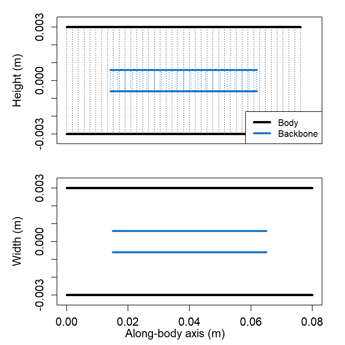
The reference example below keeps the geometry deliberately simple: a straight fluid-like body with an internal elastic cylindrical backbone offset along the body axis.

library(acousticTS)

body_shape <- cylinder(
  length_body = 0.08,
  radius_body = 0.003,
  n_segments = 40
)

backbone_shape <- cylinder(
  length_body = 0.05,
  radius_body = 0.0006,
  n_segments = 20
)

bbf_object <- bbf_generate(
  body_shape = body_shape,
  backbone_shape = backbone_shape,
  density_body = 1070,
  sound_speed_body = 1570,
  density_backbone = 1900,
  sound_speed_longitudinal_backbone = 3500,
  sound_speed_transversal_backbone = 1700,
  x_offset_backbone = 0.015
)

bbf_object <- target_strength(
  object = bbf_object,
  frequency = seq(10e3, 120e3, by = 2e3),
  model = "bbfm",
  density_sw = 1026.8,
  sound_speed_sw = 1477.3
)

head(extract(bbf_object, "model")$BBFM)

##   frequency   ka_body ka_backbone                      f_body
## 1     10000 0.1275946  0.02551893 -5.801423e-05-1.137328e-20i
## 2     12000 0.1531136  0.03062271 -8.327520e-05-1.959061e-20i
## 3     14000 0.1786325  0.03572650 -1.129211e-04-3.099232e-20i
## 4     16000 0.2041514  0.04083028 -1.468488e-04-4.606187e-20i
## 5     18000 0.2296703  0.04593407 -1.849405e-04-6.526129e-20i
## 6     20000 0.2551893  0.05103786 -2.270635e-04-8.902834e-20i
##                    f_backbone          f_backbone_aligned
## 1 -1.196018e-05+2.431034e-09i -1.196018e-05+2.431034e-09i
## 2 -1.721597e-05+5.034706e-09i -1.721597e-05+5.034706e-09i
## 3 -2.342237e-05+9.314319e-09i -2.342237e-05+9.314319e-09i
## 4 -3.057702e-05+1.586518e-08i -3.057702e-05+1.586518e-08i
## 5 -3.867731e-05+2.537004e-08i -3.867731e-05+2.537004e-08i
## 6 -4.772033e-05+3.859762e-08i -4.772033e-05+3.859762e-08i
##                          f_bs   sigma_body sigma_backbone     sigma_bs
## 1 -6.997441e-05+2.431034e-09i 3.365650e-09   1.430459e-10 4.896418e-09
## 2 -1.004912e-04+5.034706e-09i 6.934759e-09   2.963898e-10 1.009848e-08
## 3 -1.363434e-04+9.314319e-09i 1.275117e-08   5.486073e-10 1.858953e-08
## 4 -1.774259e-04+1.586518e-08i 2.156458e-08   9.349545e-10 3.147993e-08
## 5 -2.236178e-04+2.537004e-08i 3.420300e-08   1.495935e-09 5.000494e-08
## 6 -2.747838e-04+3.859762e-08i 5.155781e-08   2.277231e-09 7.550613e-08
##     TS_body TS_backbone        TS
## 1 -84.72931   -98.44524 -83.10122
## 2 -81.58969   -95.28137 -79.95744
## 3 -78.94450   -92.60738 -77.30732
## 4 -76.66259   -90.29210 -75.01966
## 5 -74.65936   -88.25087 -73.00987
## 6 -72.87706   -86.42593 -71.22018

Example outputs

Shape geometry

The shape plot below shows the body-plus-backbone composite geometry used by the reference example. The important point is that the backbone is retained as its own internal component, with its own geometry and stored offset, rather than being folded into a single effective body region.

Composite spectrum

This spectrum shows the stored BBFM output for the same reference target. The composite TS is plotted together with the component-level flesh and backbone contributions so the interference structure is visible rather than hidden.

Stored model outputs

The BBFM output table keeps the component bookkeeping explicit instead of returning only a final TS column.

Column	Meaning
frequency	Acoustic frequency in Hz
ka_body	Body acoustic size returned by the DWBA body solve
ka_backbone	Backbone acoustic size returned by the ECMS backbone solve
f_body	Flesh-body complex backscattering amplitude from DWBA
f_backbone	Backbone complex backscattering amplitude before placement
f_backbone_aligned	Backbone amplitude after centroid-based phase translation into the body frame
f_bs	Total coherent backscattering amplitude
sigma_body	Flesh-body backscattering cross-section
sigma_backbone	Aligned-backbone backscattering cross-section
sigma_bs	Total backscattering cross-section
TS_body	Flesh-body target strength
TS_backbone	Backbone target strength
TS	Total composite target strength

Those columns make it possible to inspect not just the final spectrum, but also which part of the result comes from the body, which part comes from the backbone, and how much of the composite behavior is due to coherent interference between them.

Internal consistency check

The first validation step for BBFM is to confirm that the stored composite result equals the component-wise reconstruction implied by the model design:

1. re-evaluate the flesh body as DWBA,
2. re-evaluate the backbone as ECMS,
3. apply the centroid-based phase translation, and
4. compare that explicit reconstruction against the stored BBFM output.

bbfm_out <- extract(bbf_object, "model")$BBFM

body_object <- methods::new("FLS",
  metadata = list(ID = "body"),
  model_parameters = list(),
  model = list(),
  body = extract(bbf_object, "body"),
  shape_parameters = extract(bbf_object, c("shape_parameters", "body"))
)

body_object <- target_strength(
  object = body_object,
  frequency = bbfm_out$frequency,
  model = "dwba",
  density_sw = 1026.8,
  sound_speed_sw = 1477.3
)

backbone_object <- methods::new("FLS",
  metadata = list(ID = "backbone"),
  model_parameters = list(),
  model = list(),
  body = extract(bbf_object, "backbone"),
  shape_parameters = extract(bbf_object, c("shape_parameters", "backbone"))
)

backbone_object <- target_strength(
  object = backbone_object,
  frequency = bbfm_out$frequency,
  model = "ecms",
  density_sw = 1026.8,
  sound_speed_sw = 1477.3,
  density_body = extract(bbf_object, c("backbone", "density")),
  sound_speed_longitudinal_body = extract(
    bbf_object,
    c("backbone", "sound_speed_longitudinal")
  ),
  sound_speed_transversal_body = extract(
    bbf_object,
    c("backbone", "sound_speed_transversal")
  )
)

backbone_body <- extract(backbone_object, "body")
x_center <- mean(range(backbone_body$rpos["x", ], na.rm = TRUE))
z_center <- mean(range(backbone_body$rpos["z", ], na.rm = TRUE))
phase_shift <- exp(
  2i * acousticTS::wavenumber(bbfm_out$frequency, 1477.3) *
    (x_center * cos(backbone_body$theta) + z_center * sin(backbone_body$theta))
)

reconstructed_fbs <-
  extract(body_object, "model")$DWBA$f_bs +
  extract(backbone_object, "model")$ECMS$f_bs * phase_shift

bbfm_check <- data.frame(
  frequency_kHz = bbfm_out$frequency * 1e-3,
  delta_f_bs = Mod(bbfm_out$f_bs - reconstructed_fbs),
  delta_TS_dB = bbfm_out$TS - 10 * log10(abs(reconstructed_fbs)^2)
)

knitr::kable(
  data.frame(
    quantity = c("Max $|\\Delta f_{bs}|$", "Max $|\\Delta TS|$ (dB)"),
    value = c(
      max(bbfm_check$delta_f_bs),
      max(abs(bbfm_check$delta_TS_dB))
    )
  ),
  digits = 6
)

quantity	value
Max |\Delta f_{bs}|	0
Max |\Delta TS| (dB)	0

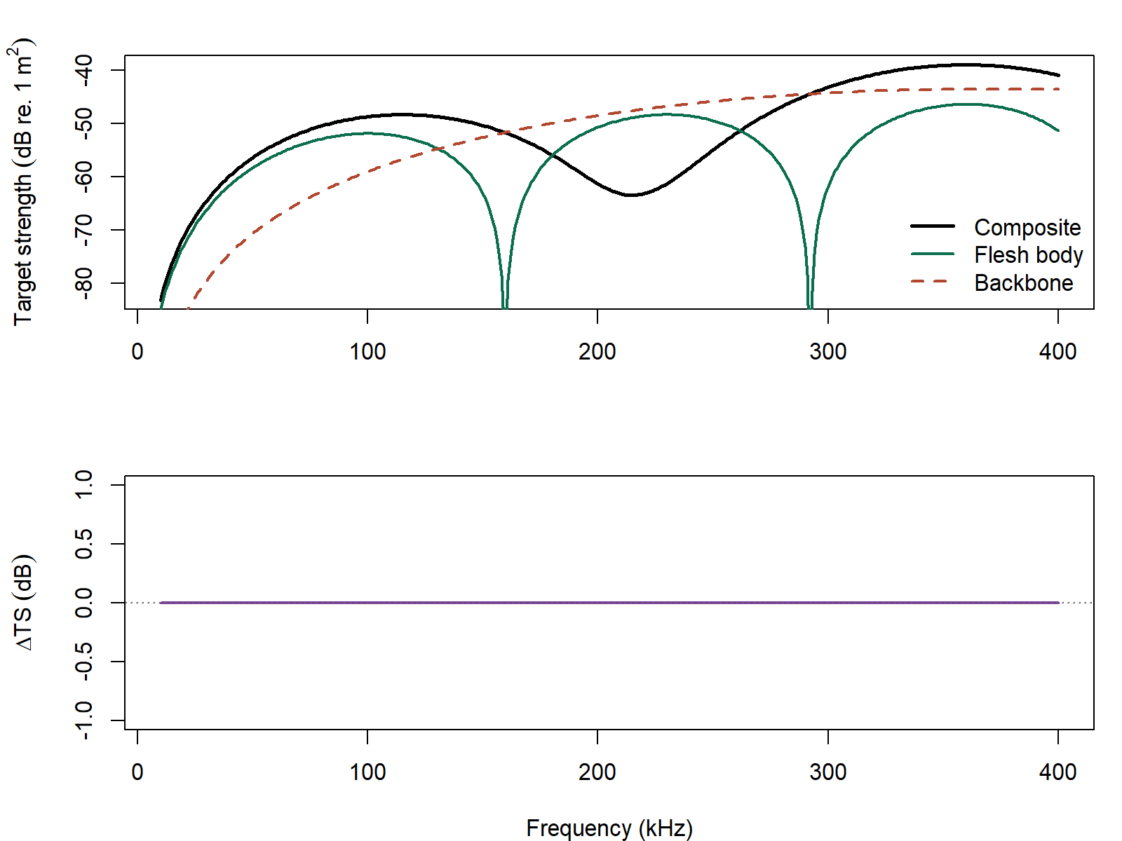
For this reconstruction check, those \Delta values should collapse to floating-point noise. That does not replace an external benchmark, but it does verify that the family is carrying out the coherent composite sum it claims to perform.

How to interpret the result

The most important interpretive point is that the final TS curve is not just the arithmetic sum of TS_body and TS_backbone. The model works in complex amplitude space:

• f_body contributes the flesh-body term,
• f_backbone_aligned contributes the backbone term after spatial placement,
• f_bs is the coherent sum of those two complex amplitudes.

That means the total TS can be:

• larger than either component alone when the phases align constructively, or
• smaller than the linear sum of the component cross-sections when the phases interfere destructively.

This is exactly why BBFM is useful. It preserves the anatomy-specific components while still letting them interfere coherently in one stored body frame.

Scope

BBFM should be interpreted as:

• a reproducible composite model for a body plus an explicit backbone,
• a convenient scaffold for swimbladder-less fish whose backbone should remain acoustically explicit,
• a first-order coherent combination model rather than a fully coupled multi-region boundary-value solve.

So the implementation answers the bookkeeping question clearly: acousticTS can construct, evaluate, and inspect this composite family in a transparent way. The remaining open work is external benchmarking and, later, more tightly coupled composite physics.

References

Clay, Clarence S., and John K. Horne. 1994. “Acoustic Models of Fish: The Atlantic Cod (Gadus Morhua).” The Journal of the Acoustical Society of America 96 (3): 1661–68. https://doi.org/10.1121/1.410245.

Gorska, Natalia, Egil Ona, and Rolf Korneliussen. 2005. “Acoustic Backscattering by Atlantic Mackerel as Being Representative of Fish That Lack a Swimbladder. Backscattering by Individual Fish.” ICES Journal of Marine Science 62 (5): 984–95. https://doi.org/10.1016/j.icesjms.2005.03.010.

Stanton, Timothy K., Dezhang Chu, Peter H. Wiebe, Linda V. Martin, and Robert L. Eastwood. 1998. “Sound Scattering by Several Zooplankton Groups. I. Experimental Determination of Dominant Scattering Mechanisms.” The Journal of the Acoustical Society of America 103 (1): 225–35. https://doi.org/10.1121/1.421469.