Viscous-elastic spherical scattering model

acousticTS implementation

Validated Experimental

These pages are motivated by layered gas-bearing fish scattering models and viscous resonance broadening (Khodabandeloo et al. 2021; Feuillade and Nero 1998).

The viscous-elastic spherical model is available through target_strength(..., model = "vesms"). The implementation is built on top of ESS objects so that the gas core and elastic shell are stored in the same object framework already used by the elastic-shelled sphere model. The additional viscous layer is then supplied through model arguments at run time.

This page focuses on a single reproducible reference case that implemented the model presented by Khodabandeloo et al. (2021) in Python. The goal is not to restate that code line by line. It is to show how the same layered target is built in acousticTS, how the model is called, and how closely the resulting spectrum matches the original implementation over a broader frequency range.

VESMS is benchmarked here against a reference Python implementation over a dense frequency sweep. That is strong across-language validation for the documented spherical case, but it is still narrower than the older modal-series families with long-standing benchmark ladders. Moreover, both implementations were authored by the same individual.

Building the reference object

The reference case uses:

gas-core radius R4 = 1.00 mm
shell outer radius R3 = 1.02 mm
shell density 1040 kg m^-3
gas density 80 kg m^-3
gas sound speed 325 m s^-1
shell shear modulus 0.2 MPa
shell bulk modulus implied by lambda = 2.4 GPa
viscous-layer density 1040 kg m^-3
viscous-layer sound speed 1510 m s^-1
viscous-layer shear and bulk viscosity both set to 3 kg m^-1 s^-1
surrounding seawater density 1027 kg m^-3
surrounding seawater sound speed 1500 m s^-1

The shell and gas core are stored in an ESS object:

library(acousticTS)

radius_gas <- 1e-3
radius_shell <- radius_gas + 0.02e-3
shear_shell <- 0.2e6
lambda_shell <- 2.4e9
bulk_shell <- lambda_shell + 2 * shear_shell / 3
sphere_shape <- sphere(radius_body = radius_shell, n_segments = 80)

vesm_object <- ess_generate(
  shape = sphere_shape,
  radius_shell = radius_shell,
  shell_thickness = radius_shell - radius_gas,
  density_shell = 1040,
  density_fluid = 80,
  sound_speed_fluid = 325,
  G = shear_shell,
  K = bulk_shell
)

Running the model

The original workflow retains the m = 0, 1, 2 terms. In acousticTS, the corresponding setting is m_limit = 2. If no outer viscous radius is supplied, VESMS estimates it from the neutral-buoyancy relation described on the theory page.

frequency <- seq(1e3, 150e3, by = 1e3)

vesm_object <- target_strength(
  object = vesm_object,
  frequency = frequency,
  model = "vesms",
  sound_speed_sw = 1500,
  density_sw = 1027,
  sound_speed_viscous = 1510,
  density_viscous = 1040,
  shear_viscosity_viscous = 3,
  bulk_viscosity_viscous = 3,
  m_limit = 2
)

head(extract(vesm_object, "model")$VESMS)

##   frequency ka_viscous    ka_shell     ka_gas                        f_bs
## 1      1000 0.01757376 0.004272566 0.00418879 -7.891754e-07-1.372246e-06i
## 2      2000 0.03514751 0.008545132 0.00837758 -3.204580e-06+5.502200e-06i
## 3      3000 0.05272127 0.012817698 0.01256637  1.445418e-05+9.321618e-08i
## 4      4000 0.07029502 0.017090264 0.01675516 -1.279015e-05-2.264936e-05i
## 5      5000 0.08786878 0.021362830 0.02094395 -2.110379e-05+3.547666e-05i
## 6      6000 0.10544253 0.025635396 0.02513274  6.057932e-05+1.028612e-06i
##       sigma_bs         TS
## 1 2.505857e-12 -116.01044
## 2 4.054354e-11 -103.92078
## 3 2.089319e-10  -96.79995
## 4 6.765813e-10  -91.69680
## 5 1.703963e-09  -87.68540
## 6 3.670912e-09  -84.35226

The stored output includes:

ka_viscous, ka_shell, and ka_gas
the complex backscattering amplitude f_bs
the linear backscattering cross-section sigma_bs
target strength TS

Validation outputs

Comparison to the original VESM implementation

For the implementation check below, the same reference geometry and material properties were run through:

acousticTS::VESMS
bespoke Python implementation

The comparison uses a shared 1-150 kHz grid with 1 kHz spacing and the same retained modal orders (m = 0, 1, 2).

After regenerating the benchmark against the current compiled acousticTS implementation, the reference case gives:

max abs. \Delta TS = 0.05598 dB
mean abs. \Delta TS = 0.00885 dB
frequency at max abs. \Delta = 60 kHz
elapsed time = 0.79 s for acousticTS and 0.98 s for the Python implementation

Comparison	N frequency	f_min (kHz)	f_max (kHz)	Max \|Δ\| TS (dB)	Mean \|Δ\| TS (dB)	f at max \|Δ\| TS (kHz)	acousticTS elapsed (s)	Python elapsed (s)
acousticTS vs original VESM	150	1	150	0.0572	0.0089	60	0.05	1.0962

The largest mismatch on this grid remains well below 0.1 dB, and the mean absolute difference stays below 0.01 dB. That is strong agreement for a layered modal-series model with complex viscous wave numbers and near-singular higher-order solves at some frequencies.

Spectrum overlay

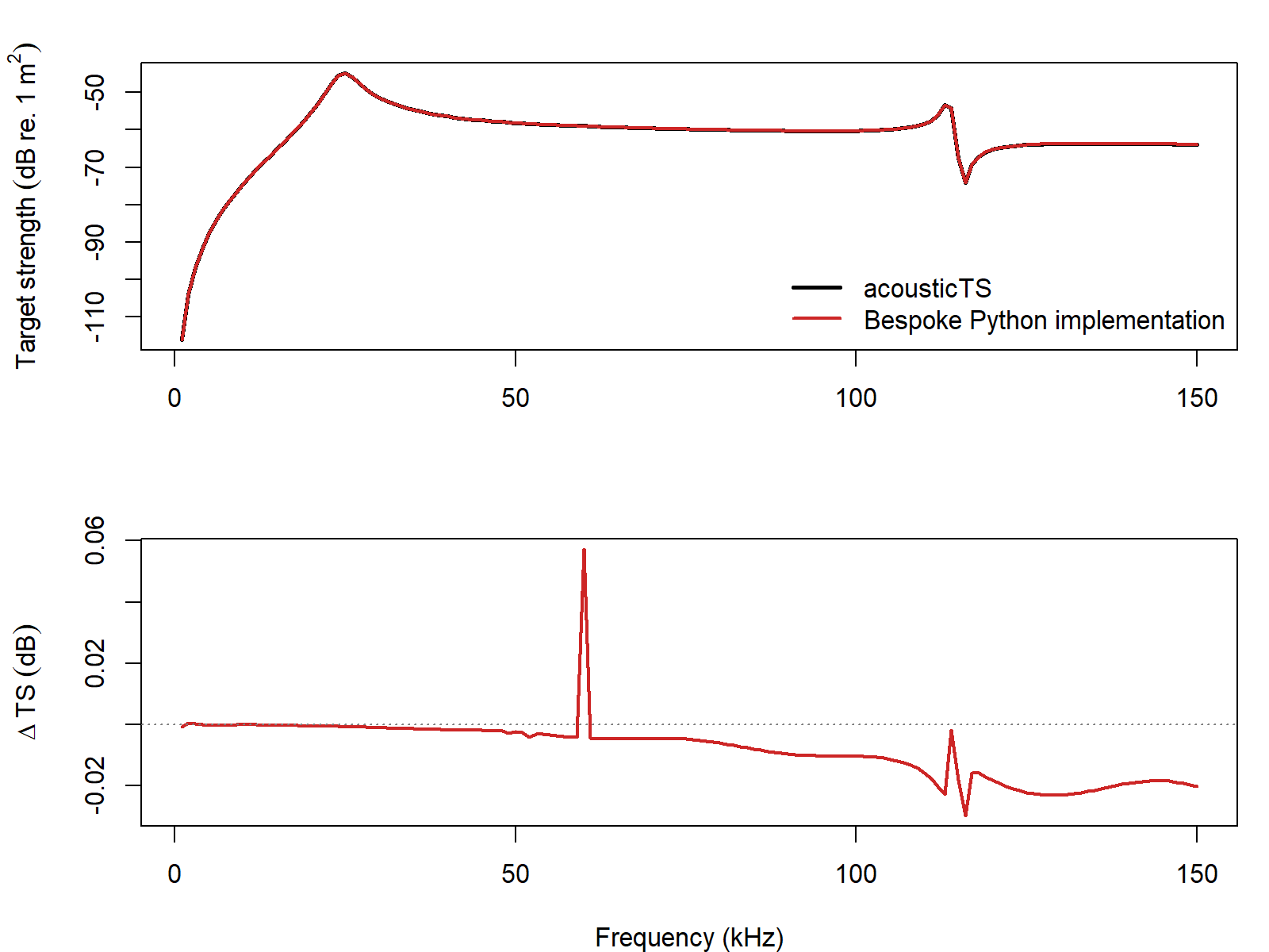
Pre-rendered VESM comparison showing the original reference spectrum, the acousticTS spectrum, and the residual across frequency.

The upper panel shows that the two spectra are visually superposed across the full comparison band. The lower panel makes the small residual drift easier to see. In this case the largest difference occurs near 60 kHz and reaches 0.05598 dB, which remains small relative to the scale of the full spectrum.

A few explicit checkpoints

	Frequency (Hz)	acousticTS TS (dB)	Python TS (dB)	Δ TS (dB)	Abs. Δ TS (dB)
1	1000	-116.01044	-116.00966	-0.00078	0.00078
38	38000	-55.81067	-55.80907	-0.00160	0.00160
60	60000	-58.93634	-58.99354	0.05720	0.05720
120	120000	-65.27321	-65.25513	-0.01807	0.01807
150	150000	-63.89102	-63.87077	-0.02025	0.02025

This comparison was run with m_limit = 2 because that is the modal content retained by the original reference implementation used here. For exploratory work at larger acoustic size, acousticTS can retain more modes by increasing m_limit or by leaving it unspecified so the model uses its default frequency-dependent cutoff.

Closing note

The implementation check is useful because the viscous-elastic model is numerically more delicate than the simpler spherical modal-series models in the package. The agreement shown here reflects the current acousticTS implementation after the compiled VESMS backend and shared complex spherical-Bessel updates, and it indicates that the model is reproducing the intended layered-reference behavior across a meaningful frequency range rather than only at a few isolated checkpoints.

References

Feuillade, C., and R. W. Nero. 1998. “A Viscous-Elastic Swimbladder Model for Describing Enhanced-Frequency Resonance Scattering from Fish.” The Journal of the Acoustical Society of America 103 (6): 3245–55. https://doi.org/10.1121/1.423076.

Khodabandeloo, Babak, Mette Dalgaard Agersted, Thor Klevjer, Gavin J. Macaulay, and Webjørn Melle. 2021. “Estimating Target Strength and Physical Characteristics of Gas-Bearing Mesopelagic Fish from Wideband in Situ Echoes Using a Viscous-Elastic Scattering Model.” The Journal of the Acoustical Society of America 149 (1): 673–91. https://doi.org/10.1121/10.0003341.