TMM implementation

acousticTS implementation

Benchmarked Partially validated Experimental

Overview Theory

These pages follow the coefficient-map view of scattering and later numerical implementations for axisymmetric bodies (Waterman 1969, 2009; Ganesh and Hawkins 2022).

The acousticTS package uses object-based scatterers, so the TMM workflow follows the same broad structure used elsewhere in the package: define the geometry, attach the material interpretation, evaluate target strength over the frequency range of interest, and then inspect the returned response carefully enough to understand what the model is actually buying you.

Why use TMM over SPHMS or PSMS?

For the supported canonical shapes, TMM is not primarily about producing a different target-strength answer from SPHMS, PSMS, or FCMS. In the exact or sanity-checked single-target cases documented here, it reduces to those shape-specific families. The reason to use TMM is that it organizes the scattering problem around an incident-to-scattered coefficient map rather than only around a monostatic backscatter formula. That makes it the natural family for stored T-matrix blocks, bistatic scattering, orientation averaging, and later multi-target workflows.

In other words:

1. if the goal is only a sphere target-strength calculation, SPHMS is the more direct exact model,
2. if the goal is only a prolate-spheroid target-strength calculation, PSMS is the more direct exact model,
3. if the goal is only a finite-cylinder target-strength calculation, FCMS is the more direct exact model even though the default monostatic cylinder branch in TMM is benchmark-matched to it, and
4. if the goal is to stay inside a transition-matrix framework that can grow into broader scattering workflows while using one common post-processing layer across spheres, spheroids, and cylinders, TMM is the relevant model family.

The TMM cylinder branch is intentionally narrower than the sphere, oblate, and prolate branches. The default monostatic path is benchmark-matched to FCMS, but full retained-angle cylinder grids and bistatic summaries remain outside the validated public scope.

Object generation

library(acousticTS)

density_sw <- 1026.8
sound_speed_sw <- 1477.3

sphere_shape <- sphere(radius_body = 0.01)
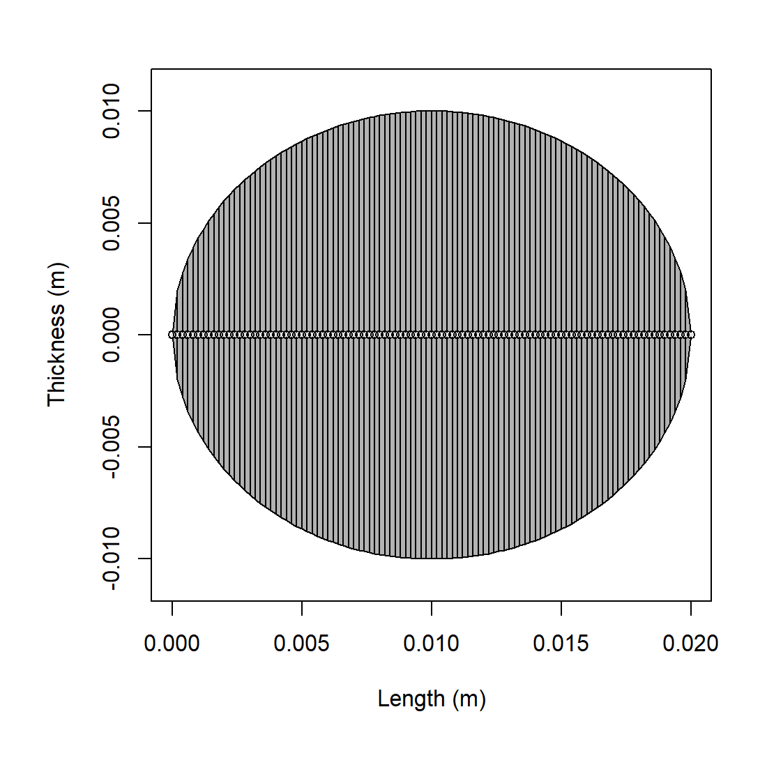
oblate_shape <- oblate_spheroid(
  length_body = 0.012,
  radius_body = 0.01,
  n_segments = 80
)
prolate_shape <- prolate_spheroid(
  length_body = 0.14,
  radius_body = 0.01,
  n_segments = 80
)
cylinder_shape <- cylinder(
  length_body = 0.07,
  radius_body = 0.01,
  n_segments = 80
)

sphere_object <- fls_generate(
  shape = sphere_shape,
  density_body = 1028.9,
  sound_speed_body = 1480.3,
  theta_body = pi / 2
)

oblate_object <- fls_generate(
  shape = oblate_shape,
  density_body = 1028.9,
  sound_speed_body = 1480.3,
  theta_body = pi / 2
)

prolate_object <- fls_generate(
  shape = prolate_shape,
  density_body = 1028.9,
  sound_speed_body = 1480.3,
  theta_body = pi / 2
)

cylinder_object <- fls_generate(
  shape = cylinder_shape,
  density_body = 1028.9,
  sound_speed_body = 1480.3,
  theta_body = pi / 2
)

The setup looks like the other exact families in the package: build a shape, generate a homogeneous scatterer, and then call target_strength(). The practical difference is that TMM keeps the calculation inside a transition-matrix viewpoint rather than only inside a direct modal-series viewpoint. The documented shape set is:

1. Sphere
2. OblateSpheroid
3. ProlateSpheroid
4. Cylinder

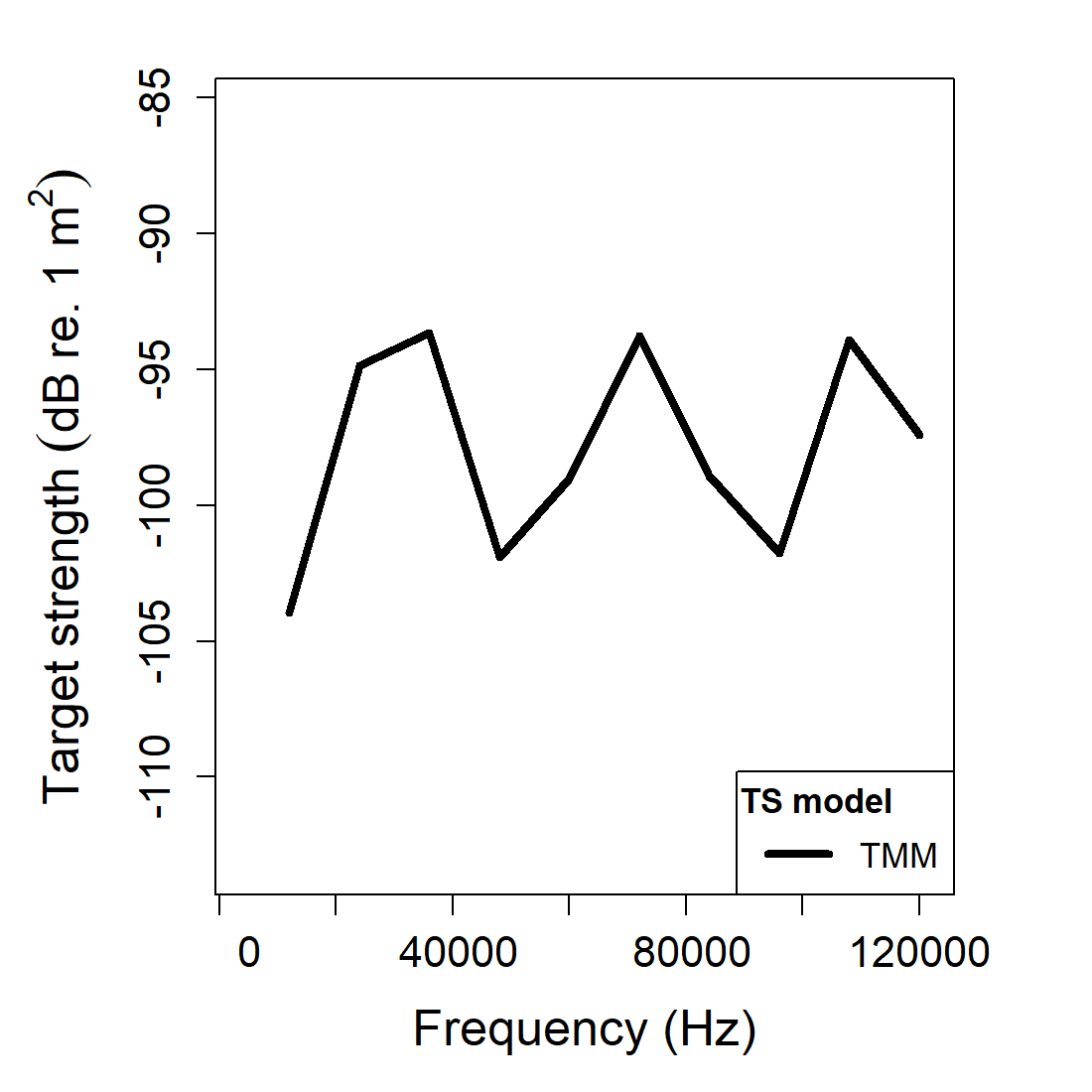
Calculating a TS-frequency spectrum

sphere_object <- target_strength(
  object = sphere_object,
  frequency = seq(12e3, 120e3, by = 12e3),
  model = "tmm",
  boundary = "liquid_filled",
  density_sw = density_sw,
  sound_speed_sw = sound_speed_sw
)

prolate_object <- target_strength(
  object = prolate_object,
  frequency = c(12e3, 18e3, 38e3, 70e3, 100e3),
  model = "tmm",
  boundary = "liquid_filled",
  density_sw = density_sw,
  sound_speed_sw = sound_speed_sw
)

sphere_object@model$TMM

##    frequency                        f_bs     sigma_bs         TS n_max
## 1      12000 -6.343290e-06+1.231703e-09i 4.023733e-11 -103.95371     6
## 2      24000 -1.805437e-05+2.830355e-08i 3.259611e-10  -94.86834     8
## 3      36000 -2.075053e-05+1.169577e-07i 4.305981e-10  -93.65928     9
## 4      48000 -8.027899e-06+1.690861e-07i 6.447575e-11 -101.90604    10
## 5      60000  1.119724e-05-1.833465e-09i 1.253781e-10  -99.01778    11
## 6      72000  2.046997e-05-3.101531e-07i 4.191160e-10  -93.77666    11
## 7      84000  1.133235e-05-3.356291e-07i 1.285348e-10  -98.90979    12
## 8      96000 -8.152309e-06+1.022055e-07i 6.647058e-11 -101.77371    13
## 9     108000 -2.017964e-05+5.314642e-07i 4.075003e-10  -93.89872    14
## 10    120000 -1.347015e-05+3.698175e-07i 1.815818e-10  -97.40928    14

prolate_object@model$TMM

##   frequency                        f_bs     sigma_bs        TS n_max
## 1     12000 -4.439503e-05+3.114131e-08i 1.970920e-09 -87.05331     4
## 2     18000 -8.709975e-05+1.363906e-07i 7.586386e-09 -81.19965     5
## 3     38000 -1.380278e-04+9.507581e-07i 1.905259e-08 -77.20046    10
## 4     70000  1.420489e-04-1.952261e-06i 2.018169e-08 -76.95042    17
## 5    100000 -9.784203e-05+1.983609e-06i 9.576997e-09 -80.18771    24

This step is intentionally similar to the other exact families. The important part is not that the call looks unfamiliar. It is that the stored result comes from a T-matrix-centered model family. For spheres, the reported n_max is the retained spherical-wave cutoff. For prolates, the reported n_max is inherited from the exact spheroidal retained system and should therefore be interpreted as the size of the retained spheroidal solve rather than as a spherical-wave truncation limit.

Extracting model results

Model results can be extracted either visually or directly through extract().

Plotting results

Accessing results

tmm_results <- extract(sphere_object, "model")$TMM
head(tmm_results)

##   frequency                        f_bs     sigma_bs         TS n_max
## 1     12000 -6.343290e-06+1.231703e-09i 4.023733e-11 -103.95371     6
## 2     24000 -1.805437e-05+2.830355e-08i 3.259611e-10  -94.86834     8
## 3     36000 -2.075053e-05+1.169577e-07i 4.305981e-10  -93.65928     9
## 4     48000 -8.027899e-06+1.690861e-07i 6.447575e-11 -101.90604    10
## 5     60000  1.119724e-05-1.833465e-09i 1.253781e-10  -99.01778    11
## 6     72000  2.046997e-05-3.101531e-07i 4.191160e-10  -93.77666    11

At this stage, the main thing to confirm is that TMM is reproducing the expected exact-family response for the chosen geometry rather than drifting away from it. That is especially important for a model family like this one, because the main value of the transition-matrix formulation is not that it should disagree with SPHMS or PSMS on canonical shapes. It is that it should reproduce them while retaining the more general transition-matrix bookkeeping.

Explicit T-matrix storage

Explicit per-frequency T-matrix block storage is available for both supported geometry branches.

sphere_store <- target_strength(
  object = fls_generate(
    shape = sphere(radius_body = 0.01, n_segments = 80),
    g_body = 1,
    h_body = 1,
    theta_body = pi / 2
  ),
  frequency = 38e3,
  model = "tmm",
  boundary = "pressure_release",
  density_sw = density_sw,
  sound_speed_sw = sound_speed_sw,
  store_t_matrix = TRUE
)

length(sphere_store@model_parameters$TMM$parameters$t_matrix[[1]])

## [1] 10

For prolate spheroids, the stored blocks live in the same @model_parameters$TMM$parameters$t_matrix slot and can be reused through helpers such as tmm_scattering(), tmm_average_orientation(), tmm_bistatic_summary(), and tmm_products() without rebuilding the retained modal solve. Cylinders can also be stored, but the retained cylinder state is intentionally narrower: it reuses the exact geometry-matched cylindrical family only for exact monostatic evaluations and orientation-averaged monostatic products. Full general-angle cylinder grids and bistatic summaries are not exposed because a validated retained cylinder angular operator is missing.

Orientation averaging from stored blocks

One of the practical reasons to keep the result in a T-matrix framework is that the same stored blocks can be reused for other single-target summaries without rerunning the boundary solve. The simplest example is an orientation-averaged monostatic cross section.

prolate_store <- target_strength(
  object = fls_generate(
    shape = prolate_spheroid(
      length_body = 0.14,
      radius_body = 0.01,
      n_segments = 80
    ),
    density_body = 1028.9,
    sound_speed_body = 1480.3,
    theta_body = pi / 2
  ),
  frequency = seq(12e3, 100e3, 2e3),
  model = "tmm",
  boundary = "liquid_filled",
  density_sw = density_sw,
  sound_speed_sw = sound_speed_sw,
  store_t_matrix = TRUE
)

orientation_dist <- tmm_orientation_distribution(
  distribution = "uniform",
  lower = 0.45 * pi,
  upper = pi,
  n_theta = 7
)

orientation_avg <- tmm_average_orientation(
  object = prolate_store,
  distribution = orientation_dist
)

orientation_avg

##    frequency     sigma_bs         TS
## 1      12000 4.502163e-10  -93.46579
## 2      14000 6.702413e-10  -91.73769
## 3      16000 9.192786e-10  -90.36553
## 4      18000 1.170862e-09  -89.31494
## 5      20000 1.399276e-09  -88.54097
## 6      22000 1.548806e-09  -88.10003
## 7      24000 1.585990e-09  -87.99700
## 8      26000 1.469957e-09  -88.32695
## 9      28000 1.232136e-09  -89.09341
## 10     30000 9.347098e-10  -90.29323
## 11     32000 6.301750e-10  -92.00539
## 12     34000 3.607924e-10  -94.42743
## 13     36000 1.701901e-10  -97.69066
## 14     38000 8.946596e-11 -100.48342
## 15     40000 1.192773e-10  -99.23442
## 16     42000 2.704566e-10  -95.67902
## 17     44000 5.266602e-10  -92.78470
## 18     46000 8.330752e-10  -90.79316
## 19     48000 1.119975e-09  -89.50792
## 20     50000 1.305324e-09  -88.84282
## 21     52000 1.354505e-09  -88.68219
## 22     54000 1.285562e-09  -88.90907
## 23     56000 1.118337e-09  -89.51427
## 24     58000 8.827687e-10  -90.54153
## 25     60000 6.240222e-10  -92.04800
## 26     62000 3.913264e-10  -94.07461
## 27     64000 2.144002e-10  -96.68775
## 28     66000 1.343882e-10  -98.71639
## 29     68000 1.862644e-10  -97.29870
## 30     70000 3.663744e-10  -94.36075
## 31     72000 6.192308e-10  -92.08147
## 32     74000 8.730832e-10  -90.58944
## 33     76000 1.074125e-09  -89.68945
## 34     78000 1.193339e-09  -89.23236
## 35     80000 1.223384e-09  -89.12437
## 36     82000 1.161184e-09  -89.35099
## 37     84000 1.016937e-09  -89.92706
## 38     86000 8.210382e-10  -90.85637
## 39     88000 5.984286e-10  -92.22988
## 40     90000 3.856175e-10  -94.13843
## 41     92000 2.527349e-10  -95.97335
## 42     94000 2.403773e-10  -96.19107
## 43     96000 3.303472e-10  -94.81029
## 44     98000 4.884121e-10  -93.11214
## 45    100000 6.738344e-10  -91.71447

By default, tmm_average_orientation() assumes the exact monostatic receive direction for each supplied incident angle. So the helper is averaging the differential backscattering cross section over the chosen orientation distribution, not rebuilding the underlying T-matrix solve at every angle.

The distribution helper is there so the main orientation pathways stay explicit and standardized:

1. distribution = "uniform" creates a uniform distribution in theta_body over a bounded interval,
2. distribution = "normal" creates a normal distribution on [0, pi],
3. distribution = "truncated_normal" creates a normal distribution restricted to [lower, upper], and
4. distribution = "quadrature" or distribution = "pdf" lets the user supply their own angle grid and either direct weights or a density.

Because this helper is meant for monostatic orientation-averaged backscatter, its returned columns follow the same naming convention used elsewhere in the package: sigma_bs and TS.

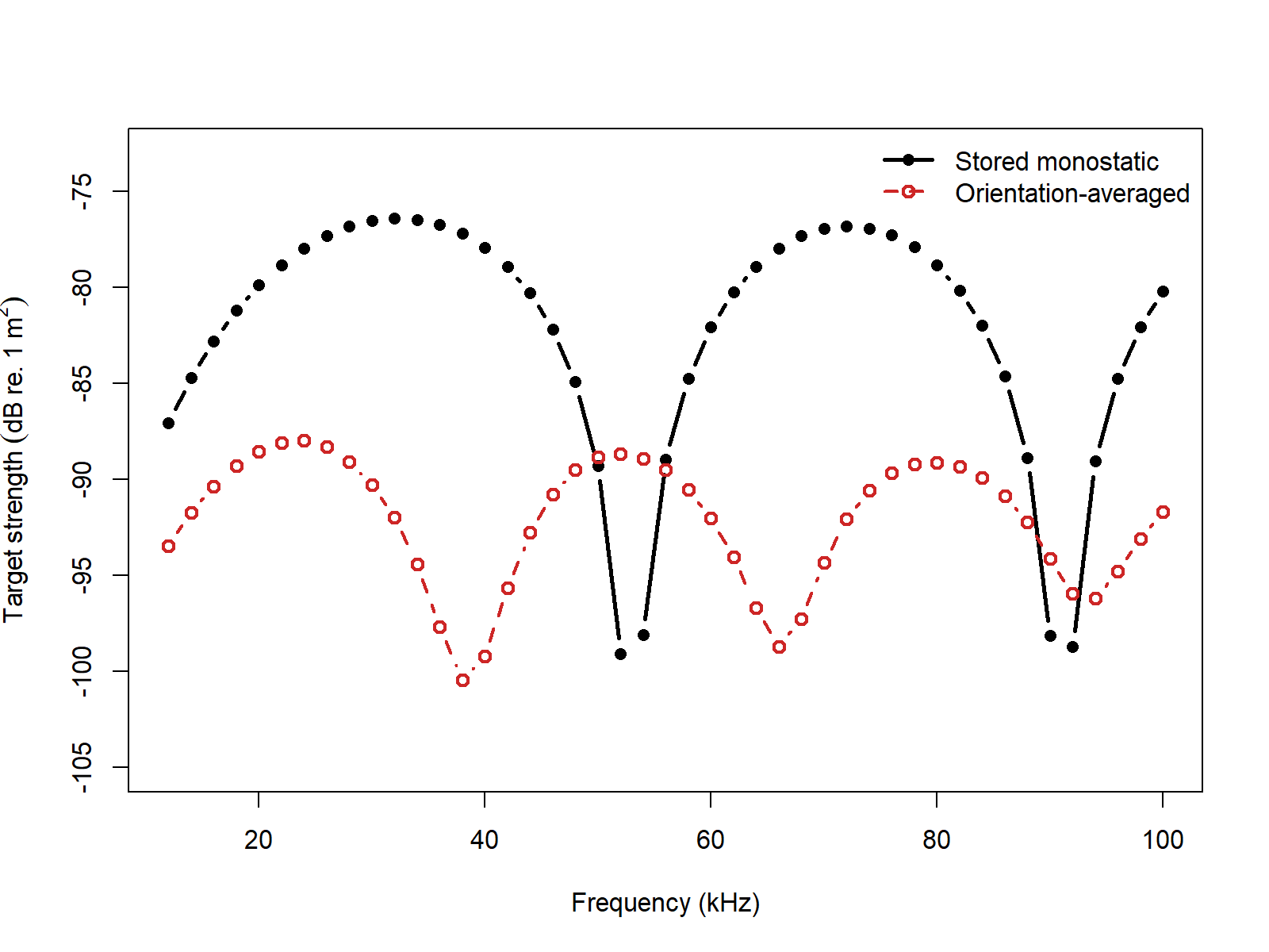
The orientation-averaged line can sit far below the stored monostatic line, and that is not a bug by itself. The stored monostatic spectrum in this example is the broadside response of one fixed orientation, while the orientation-averaged spectrum is a linear average of sigma_bs over a wide range of body angles. For a long prolate spheroid, broadside is typically much stronger than the more oblique and near-end-on views, so the average can be many decibels lower than the broadside-only curve.

Angular scattering slices from stored blocks

The same stored blocks can also be sent through plot(..., type = "scattering") to inspect a single angular slice of the far-field response at a chosen stored frequency.

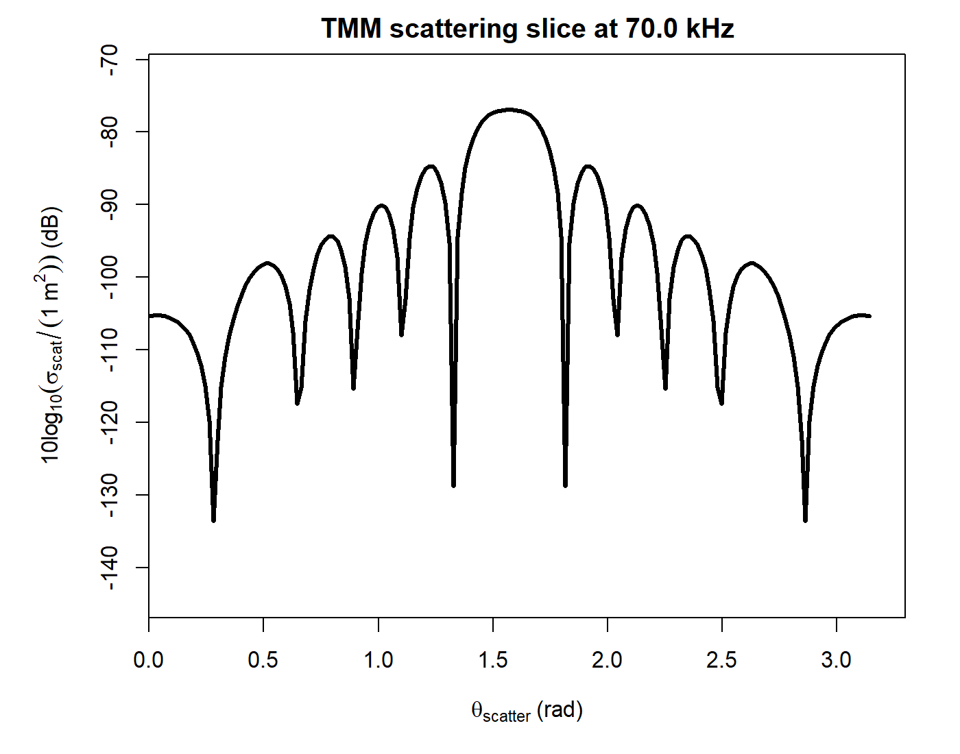
This is useful when the question is no longer just “what is the monostatic target strength?” but also “how does the same stored transition matrix distribute scattering over receive angle at a fixed frequency?” That is exactly the kind of post-processing that is natural in a T-matrix workflow and comparatively awkward in the purely direct exact-family formulations.

All of the tmm_scattering()-style helpers use the body-fixed angular coordinates of the canonical axisymmetric target, not arbitrary world-frame directions. For the built-in prolate, oblate, and cylinder shapes in acousticTS, the symmetry axis is the body x-axis. So when these helpers are compared against an external BEM/FEM slice generated in a world x-y plane, the world directions need to be converted to the body-fixed (\theta, \phi) convention before the comparison is apples-to-apples.

Higher-level bistatic summaries

Once the stored blocks are available, the next natural step is to move beyond individual points and slices and ask for higher-level bistatic summaries. Within the documented package scope, that applies to the spherical and spheroidal stored branches. tmm_bistatic_summary() does that for one stored frequency by returning:

1. a forward-centered great-circle slice,
2. an orthogonal dorsal/ventral-style great-circle slice,
3. the peak-scattering direction on a 2D receive-angle grid,
4. the exact monostatic backscatter value,
5. a -3 dB backscatter-lobe width measured on the forward-centered slice, and
6. integrated scattering over coarse angular sectors measured relative to the forward direction.

summary_70 <- tmm_bistatic_summary(
  object = prolate_store,
  frequency = 70e3,
  n_theta = 21,
  n_phi = 41,
  n_psi = 41
)

summary_70$metrics

##   frequency forward_sigma_scat forward_sigma_scat_dB     sigma_bs        TS
## 1     70000        7.00483e-07             -61.54602 2.018169e-08 -76.95042
##   peak_theta_scatter peak_phi_scatter peak_psi_scatter peak_sigma_scat
## 1           1.570796         3.141593                0     7.00483e-07
##   peak_sigma_scat_dB backscatter_lobe_width
## 1          -61.54602               1.021018

summary_70$sector_integrals

##            sector  psi_min  psi_max integrated_sigma_scat
## 1  forward_sector 0.000000 1.047198          1.711232e-07
## 2  oblique_sector 1.047198 2.094395          1.659806e-08
## 3 backward_sector 2.094395 3.141593          1.427224e-08

Those summary products are not new physics. They are just structured reuses of the same stored T-matrix blocks. That makes them a good sanity-check layer: the exact monostatic value reported by summary_70$metrics$TS should agree with the monostatic TS already stored on the object at 70 kHz.

Single solved target, many post-process products

The separate helpers are useful when only one post-processing product is needed. But the broader T-matrix workflow is often “solve once, then ask for several things.” The higher-level tmm_products() wrapper is meant for exactly that pattern.

products_70 <- tmm_products(
  object = prolate_store,
  frequency = 70e3,
  orientation = orientation_dist,
  bistatic_summary = TRUE,
  n_theta = 21,
  n_phi = 41,
  n_psi = 41
)

names(products_70)

## [1] "monostatic"          "orientation_average" "bistatic_summary"

products_70$bistatic_summary$metrics

##   frequency forward_sigma_scat forward_sigma_scat_dB     sigma_bs        TS
## 1     70000        7.00483e-07             -61.54602 2.018169e-08 -76.95042
##   peak_theta_scatter peak_phi_scatter peak_psi_scatter peak_sigma_scat
## 1           1.570796         3.141593                0     7.00483e-07
##   peak_sigma_scat_dB backscatter_lobe_width
## 1          -61.54602               1.021018

This is closer to the real reason for keeping a T-matrix-based representation around. The workflow is no longer “get one monostatic spectrum and stop.” It becomes “solve the target once, then reuse the stored operator for monostatic, orientation-averaged, and bistatic products.”

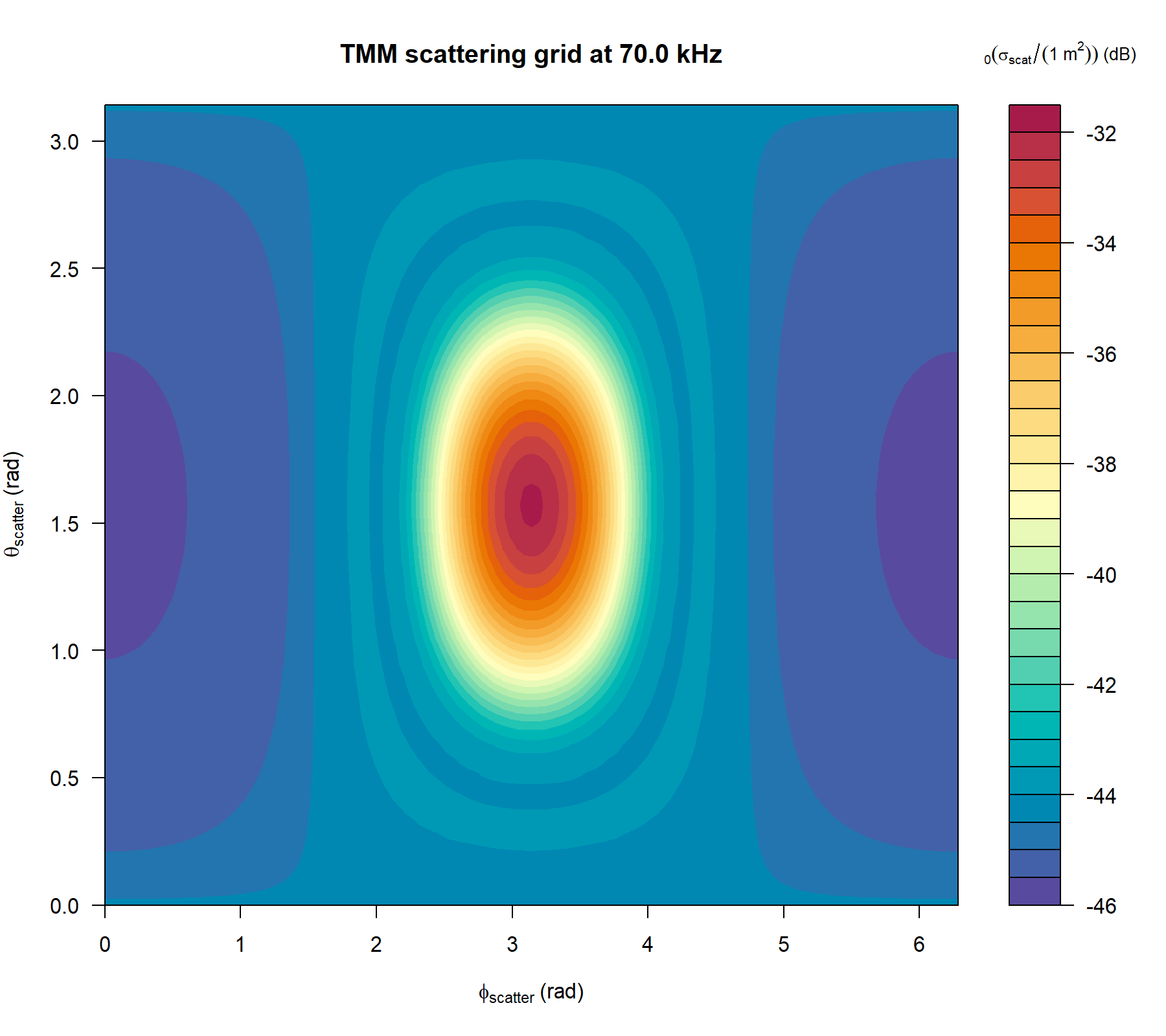
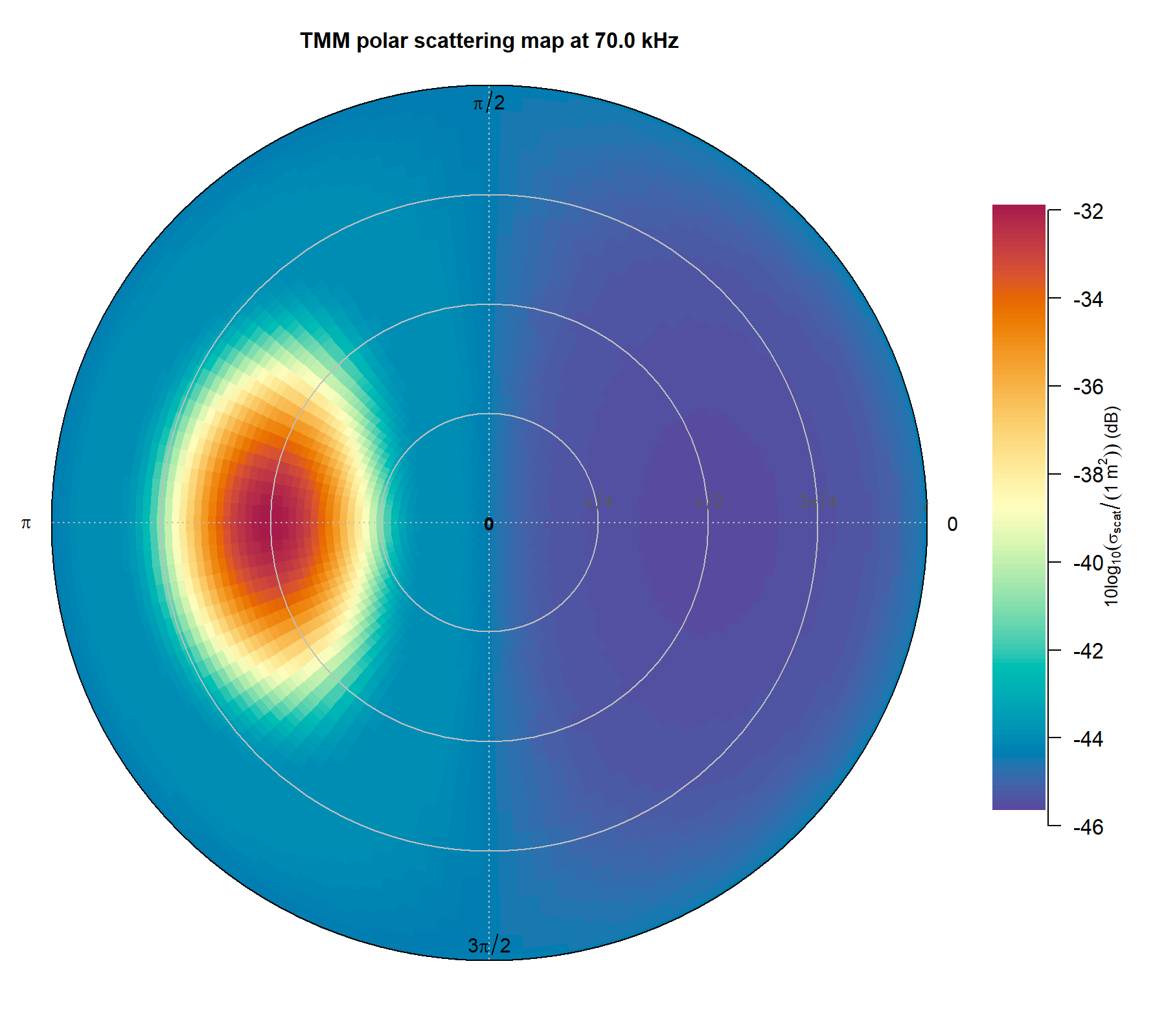
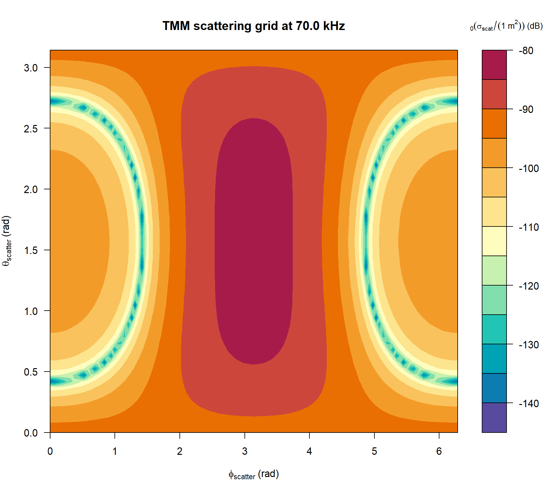
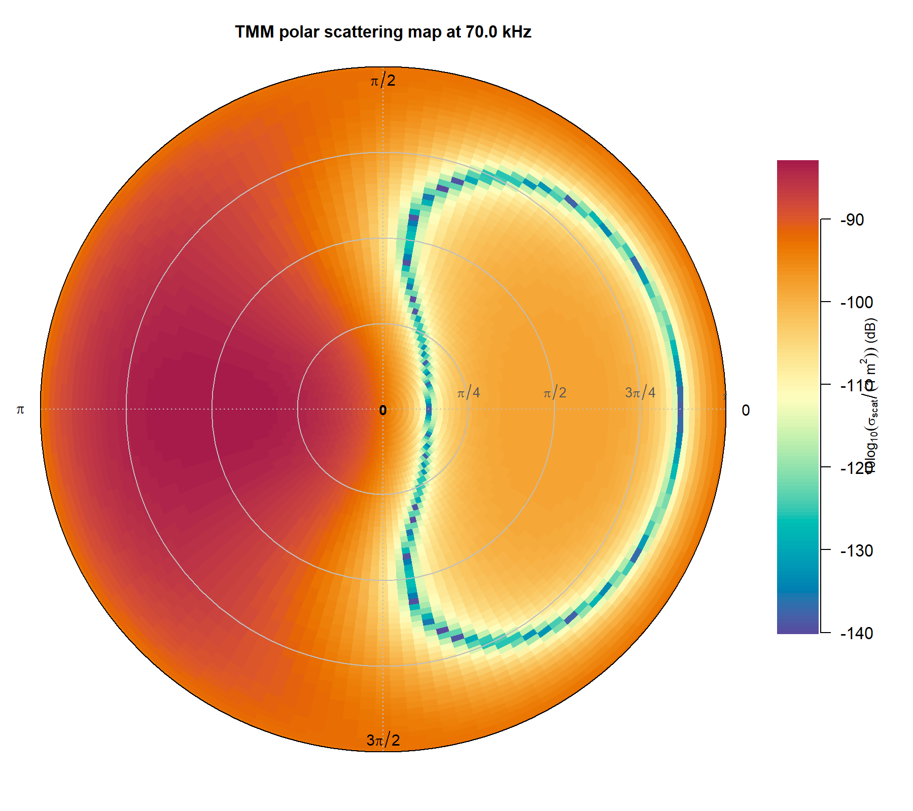
Bistatic scattering grids and polar maps

For two-dimensional receive-angle views, the stored blocks can be reused through tmm_scattering_grid() or displayed directly through plot(..., type = "scattering", polar = TRUE) or plot(..., type = "scattering", heatmap = TRUE). The implementation page uses pre-rendered figures for those heavier views so the article stays lightweight to build.

The vignette embeds pre-rendered examples here so the implementation page does not need to rebuild the heavier two-dimensional scattering figures every time it is rendered. The gallery covers the stored branches that actually support angular grids: Sphere, OblateSpheroid, and ProlateSpheroid. Cylinder is intentionally omitted because the retained-cylinder path stops at exact monostatic reuse and orientation-averaged monostatic products.

Shape gallery

• Sphere
• Oblate
• Prolate

These two views show the stored pressure-release sphere at 70 kHz. The heatmap uses the direct (\phi_\text{scatter}, \theta_\text{scatter}) grid, while the polar map wraps the same grid into a circular view.

These two views show the stored liquid-filled oblate spheroid at 70 kHz, which is a useful intermediate case because it still uses the spherical-coordinate retained branch but no longer has the exact spherical symmetry of the sphere.

These two views show the stored liquid-filled prolate spheroid at 70 kHz, which is the geometry where the retained spheroidal angular operator is most directly useful.

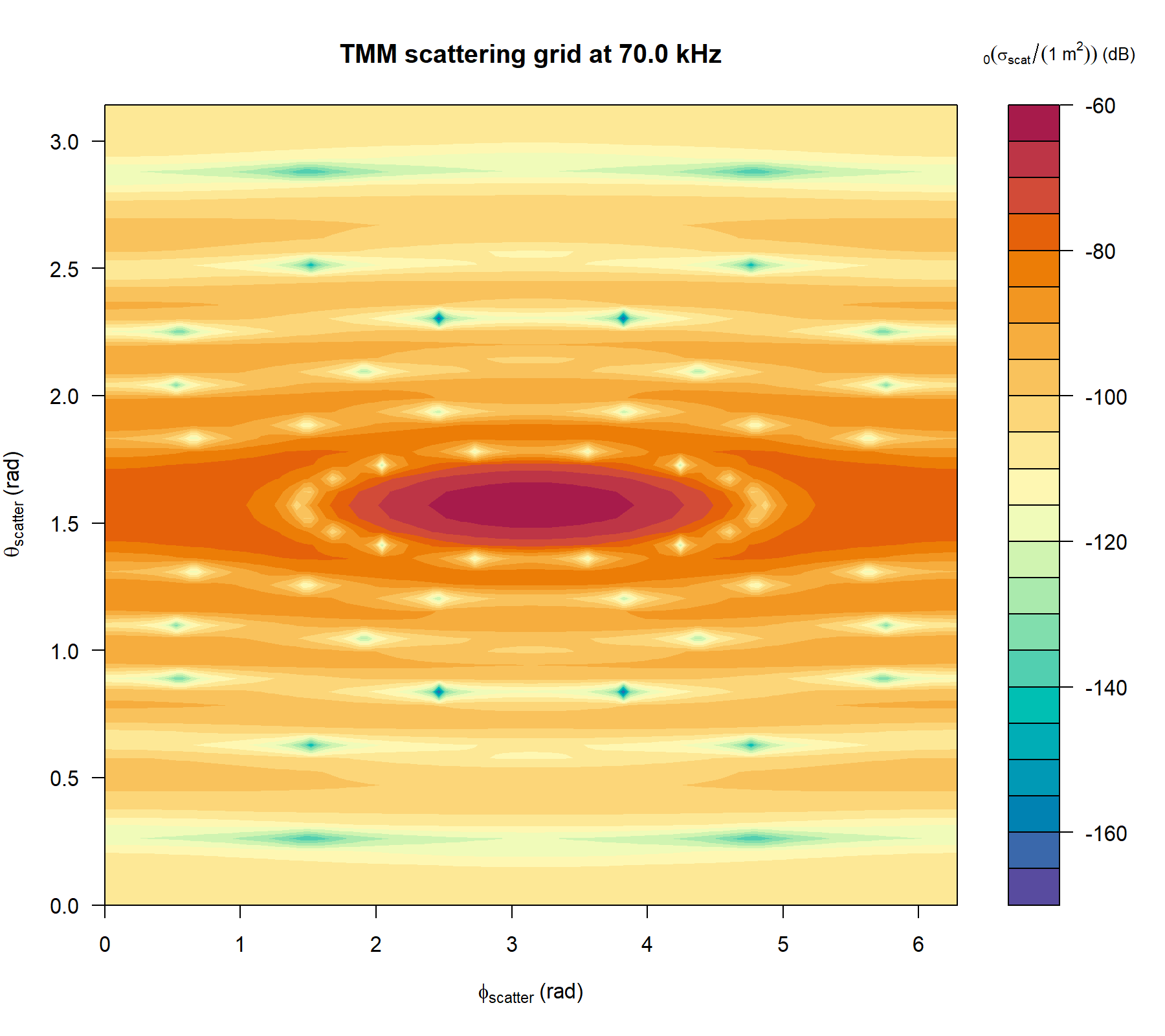
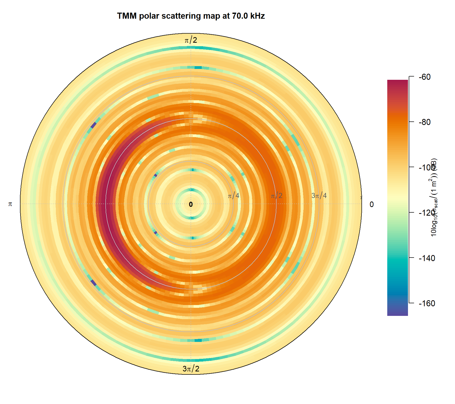
In each polar view, the radius is the scattering polar angle theta_scatter, not physical distance from the target. So the center corresponds to theta_scatter = 0, the outer ring corresponds to theta_scatter = pi, and the target itself is not drawn as a literal object at the origin.

Benchmark comparisons

The benchmark ladder is intentionally shape-specific and follows the exact-family references already used elsewhere in the package.

• Sphere cases are compared against SPHMS
• Oblate spheroids are checked through both the exact sphere limit and an external pressure-release BEMPP far-field slice for a genuinely nonspherical oblate case
• Prolate spheroid cases are compared against PSMS
• Cylinder cases are compared against FCMS for the default monostatic branch over the tested 12-200 kHz grids

Those broad checks were run over multiple shapes and multiple frequency grids rather than just one canonical example, but the resulting summary tables are kept static here so the implementation page remains lightweight to build.

Benchmark tables

• Sphere
• Oblate
• Prolate
• Cylinder

Spherical models were benchmarked against SPHMS over 12:120 by 4 kHz for a = 5, 10, and 18 mm.

a (mm)	Boundary	\max \vert \Delta TS \vert ~ (\text{dB})	\vert \overline{\Delta TS} \vert ~ (\text{dB})	t_\text{TMM} (\text{s})	t_\text{SPHMS} (\text{s})
5	fixed_rigid	1.66e-11	1.95e-12	0.27	0.03
5	pressure_release	1.76e-11	1.77e-12	0.31	0.07
5	liquid_filled	2.26e-11	4.04e-12	0.39	0.01
5	gas_filled	1.75e-11	1.75e-12	0.47	0.03
10	fixed_rigid	2.37e-10	2.75e-11	0.50	0.00
10	pressure_release	2.44e-10	2.91e-11	0.56	0.02
10	liquid_filled	1.14e-10	1.67e-11	0.75	0.02
10	gas_filled	2.45e-10	2.86e-11	0.78	0.01
18	fixed_rigid	7.62e-10	8.32e-11	1.03	0.01
18	pressure_release	7.91e-10	8.49e-11	1.06	0.00
18	liquid_filled	4.59e-09	2.36e-10	1.47	0.02
18	gas_filled	8.46e-10	8.71e-11	1.53	0.00

Oblate sphere-limit checks used three equal-volume radii and compared against the SPHMS sphere limit at 12, 38, 70, and 120 kHz.

Boundary	\max \vert \Delta TS \vert ~ (\text{dB})	\vert \overline{\Delta TS} \vert ~ (\text{dB})	t_\text{TMM} (\text{s})	t_\text{SPHMS} (\text{s})
fixed_rigid	3.60e-10	4.97e-11	0.11	0.05
pressure_release	3.12e-10	5.06e-11	0.12	0.00
liquid_filled	1.04e-10	2.02e-11	0.15	0.02
gas_filled	3.12e-10	5.07e-11	0.23	0.00

Prolate models were benchmarked against PSMS. The 60 x 8 mm case used 12, 18, 38, 70, 100, and 150 kHz, while the 140 x 10 mm case used 12, 18, 38, 70, and 100 kHz.

L (mm)	a (mm)	Boundary	\max \vert \Delta TS \vert ~ (\text{dB})	\vert \overline{\Delta TS} \vert ~ (\text{dB})	t_\text{TMM} (\text{s})	t_\text{PSMS} (\text{s})
60	8	fixed_rigid	0.00000	0.00000	0.03	0.08
60	8	pressure_release	0.00000	0.00000	0.03	0.02
60	8	liquid_filled	0.00000	0.00000	2.50	1.83
60	8	gas_filled	0.00000	0.00000	2.39	2.53
140	10	fixed_rigid	0.00000	0.00000	0.03	0.02
140	10	pressure_release	0.00000	0.00000	0.02	0.02
140	10	liquid_filled	0.00000	0.00000	2.81	2.23
140	10	gas_filled	0.00000	0.00000	2.70	2.81

Cylinders were benchmarked against FCMS over 12, 18, 38, 70, 100, 150, and 200 kHz.

L (mm)	a (mm)	Boundary	\max \vert \Delta TS \vert ~ (\text{dB})	\vert \overline{\Delta TS} \vert ~ (\text{dB})	t_\text{TMM} (\text{s})	t_\text{FCMS} (\text{s})
70	10	fixed_rigid	0.00e+00	0.00e+00	0.011	0.004
70	10	pressure_release	0.00e+00	0.00e+00	0.001	0.000
70	10	liquid_filled	0.00e+00	0.00e+00	0.009	0.001
70	10	gas_filled	0.00e+00	0.00e+00	0.002	0.004
50	8	fixed_rigid	3.55e-15	5.08e-16	0.000	0.000
50	8	pressure_release	0.00e+00	0.00e+00	0.001	0.000
50	8	liquid_filled	0.00e+00	0.00e+00	0.004	0.001
50	8	gas_filled	0.00e+00	0.00e+00	0.002	0.004

These are intentionally not one-off canonical checks. The tables above sweep multiple shapes and frequency sets so the agreement is not just tied to one hand-picked sphere or one hand-picked prolate spheroid.

Two points matter most here.

1. The sphere branch behaves like a true spherical-coordinate T-matrix implementation and agrees with SPHMS to numerical precision on the tested grid.
2. The oblate branch collapses correctly onto the exact sphere solution in the sphere limit and also agrees closely with an external pressure-release BEMPP slice for a genuinely nonspherical oblate case.
3. The prolate branch uses the geometry-matched spheroidal-coordinate backend, so the TMM and PSMS spectra coincide across the tested geometry and frequency sweep for all four supported scalar boundary types.
4. The default monostatic finite-cylinder branch lands directly on FCMS across the tested geometry and frequency sweep because it uses the geometry-matched cylindrical modal backend, and the stored-cylinder path reuses that same backend only where the monostatic mapping is exact.

That fourth point is an in-package exact-family consistency check, not a claim that the cylinder branch is already externally closed against BEM/FEM over all angles. It means the default monostatic TMM cylinder branch and FCMS are the same calculation family at the package level. The external cylinder discussion below is separate and is the reason the retained general-angle cylinder helpers remain disabled.

That benchmark pattern is exactly what one would want at this stage. The TMM family is useful because it stays within a transition-matrix formulation while landing on the correct exact-family answers for the canonical geometries it supports in the default monostatic workflow.

Diagnostics and internal validation

Exact-family comparisons are the first validation ladder, but they are not the whole story for TMM. For the newer branches, it is also useful to check whether the retained operator is internally self-consistent. The tmm_diagnostics() helper does that by reusing the stored blocks and reporting:

1. monostatic reconstruction residuals,
2. reciprocity residuals under incident/receive-angle exchange,
3. an optical-theorem residual for the spherical-coordinate branch, and
4. block-level conditioning summaries.

For the rigid and pressure-release prolate branches, the stored-block TMM angular field can be checked directly against the exact general-angle spheroidal modal-series solution used by PSMS. That is the fastest way to constrain off-axis disagreements, because it removes external meshing and solver conventions from the loop and asks only whether the retained prolate operator reproduces the exact scalar spheroidal field at the same incident and receive angles.

diag_70 <- tmm_diagnostics(
  prolate_store,
  n_theta = 31,
  n_phi = 61
)

diag_70$summary

Independent BEMPP cross-checks were available for the pressure-release sphere, oblate, and prolate branches. The cylinder situation is different because the retained-cylinder scope is intentionally monostatic-only. So the validation ladder for these branches combines:

1. exact-family checks where they exist (SPHMS, PSMS, FCMS),
2. limiting-case checks such as the oblate sphere limit, and
3. theorem-based diagnostics from the stored T-matrix blocks.

The table below shows representative diagnostic summaries for one stored object from each supported branch, where e is the residual.

Case	\mathscr{f}~(\text{kHz})	Max monostatic e	Max reciprocity e	Max optical-theorem e	Min block rcond	Max block transpose e
sphere, fixed_rigid	38, 70	2.55e-16	2.12e-16	1.24e-03	3.11e-09	1.93e-16
oblate spheroid, liquid_filled	38, 70	2.80e-16	1.14e-04	1.34e-03	2.24e-16	3.48e-01
prolate spheroid, liquid_filled	38, 70	3.28e-16	2.64e-12	NA	3.35e-47	1.15e-13
finite cylinder, fixed_rigid	38, 70	0.00e+00	NA	NA	NA	NA

Two points are worth emphasizing.

1. The sphere and prolate branches are numerically self-consistent to essentially machine precision on the tested grids.
2. The stored-cylinder branch is deliberately narrower than the sphere and prolate branches. It carries only the geometry-matched monostatic reuse path, so reciprocity and optical-theorem-style angular diagnostics are left as NA rather than being computed from an unvalidated cylinder grid operator.

Sphere-to-spheroid continuation

For spheroidal targets, one of the most useful internal checks is to start from the equal-volume sphere limit and then deform the target smoothly to the requested aspect ratio. The monostatic response should move smoothly along that path. Abrupt jumps, non-finite values, or strong zig-zag second differences at modest aspect ratio are a sign that the truncation or angular reconstruction is not under control.

This check is built into tmm_diagnostics() for prolate and oblate targets. The continuation is generated at constant volume, beginning from the exact sphere limit and stepping to the requested spheroidal aspect ratio.

The figure below shows the built-in continuation path for a pressure-release prolate spheroid with target aspect ratio 3.5.

Sphere-to-spheroid continuation path for a pressure-release prolate spheroid. The exact sphere limit is at aspect ratio 1, and the target spheroid is at aspect ratio 3.5.

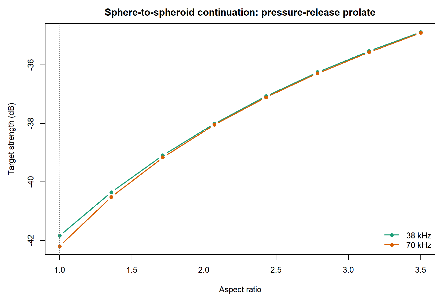
The practical point is simple: this is a much faster development check than an external solver loop. It constrains whether the stored T-matrix branch behaves sensibly before external meshing, field normalization, or far-field extraction are even involved.

Exact prolate angular validation

For the retained prolate branch, the most useful validation is not a paper-style sketch and not an external mesh-based comparison. It is a direct check against the exact general-angle spheroidal solution already available in the package for rigid and pressure-release scalar prolates. That is the right apples-to-apples comparison because it uses:

1. the same geometry,
2. the same incident and receive-angle definitions,
3. the same scalar boundary conditions, and
4. the same far-field normalization.

So, for the retained prolate TMM operator, the key question is simply whether tmm_scattering() reproduces the exact prolate_spheroid_fbs() field when both are evaluated at the same stored frequency and the same incident/receive angles.

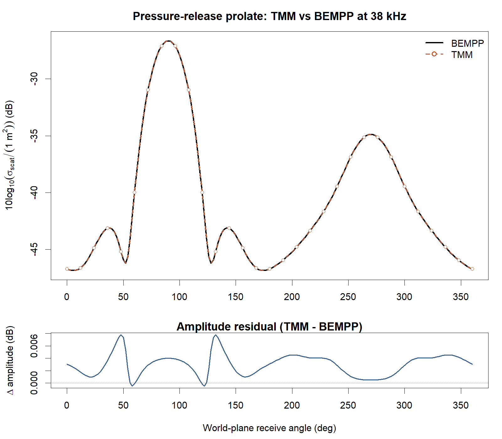
The figure below shows that check for a rigid and a pressure-release prolate spheroid with L = 70 mm, a = 10 mm, broadside incidence, and a 38 kHz equatorial receive-angle sweep. The line is the exact general-angle spheroidal solution and the open symbols are the stored-block TMM reconstruction.

Exact-vs-stored validation for rigid and pressure-release prolate spheroids at 38 kHz, shown as equatorial receive-angle sweeps under broadside incidence.

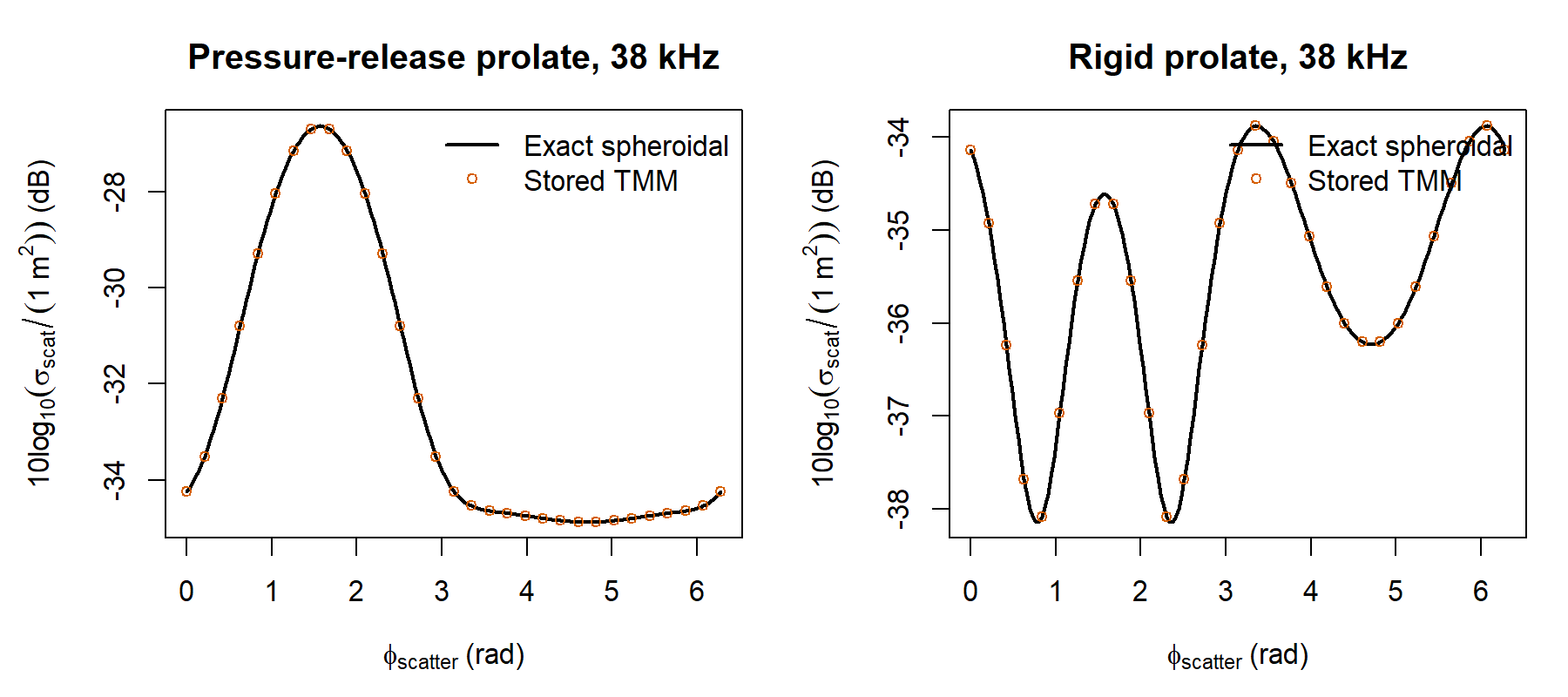
This directly tests the retained angular operator that powers tmm_scattering(), tmm_scattering_grid(), and the higher-level post-processing helpers.

That body-fixed angle convention also resolves the mismatch with the exploratory BEMPP prolate slice.

External comparison tables

• Prolate
• Oblate
• Cylinder

For the pressure-release prolate case with L = 70 mm, a = 10 mm, and 38 kHz, the retained TMM branch and the external BEMPP far-field solution line up closely across the tested incidence angles:

World-frame incidence (deg)	Max abs. \Delta amplitude (dB)	Mean abs. \Delta amplitude (dB)	Note
0	0.0069	0.0033	pressure-release, BEMPP far-field
45	0.0076	0.0031	pressure-release, BEMPP far-field
90	0.0078	0.0030	pressure-release, BEMPP far-field

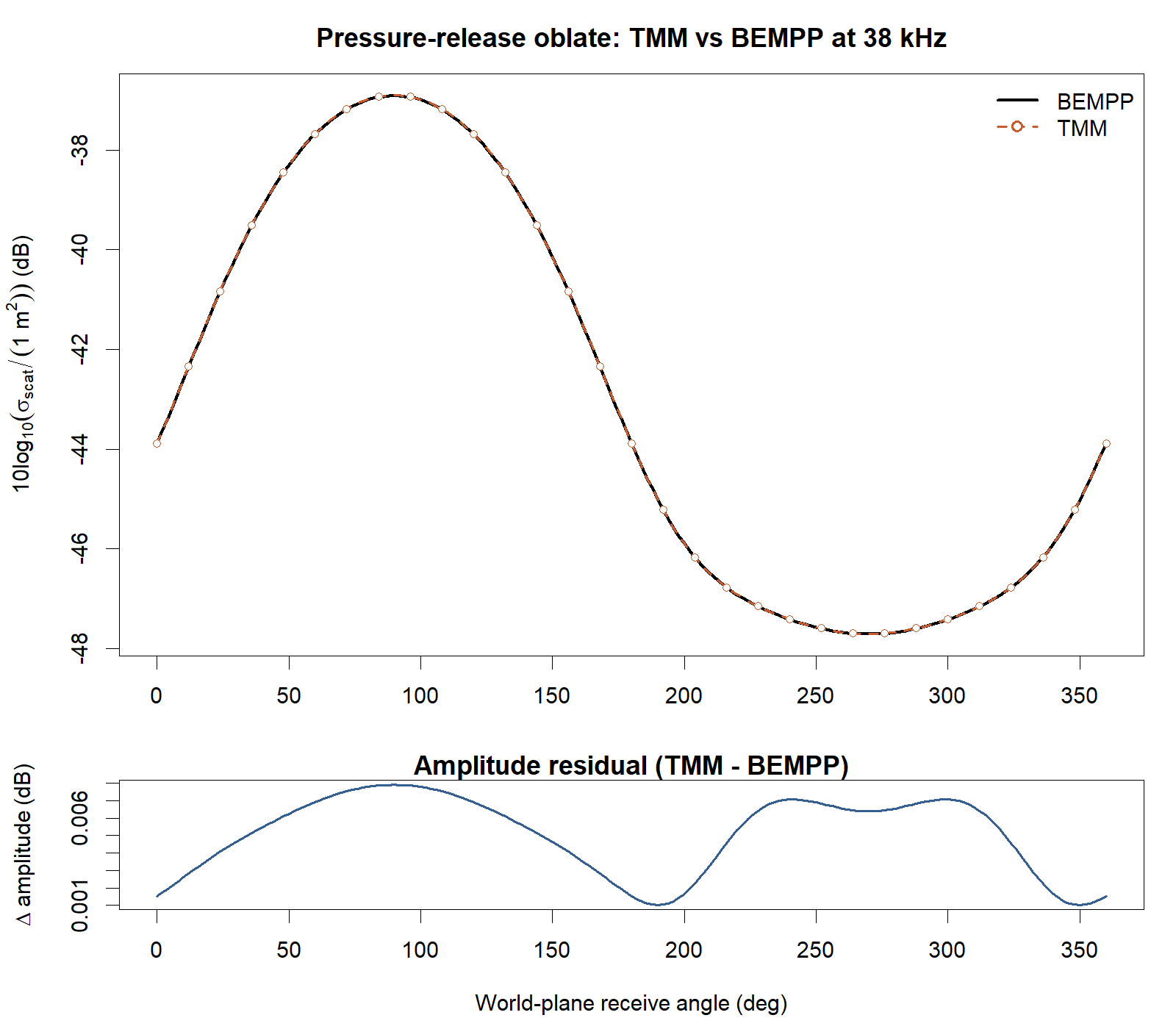
The same body-fixed/world-frame conversion is also important for the nonspherical oblate branch, which uses the spherical-coordinate retained operator. For a pressure-release oblate with polar semiaxis c = 6 mm and equatorial semiaxis a = 10 mm, the corrected BEMPP comparison is likewise tight on the tested cases:

Frequency (kHz)	World-frame incidence (deg)	Max abs. \Delta amplitude (dB)	Mean abs. \Delta amplitude (dB)	Validation note
38	0	0.0091	0.0054	pressure-release, BEMPP far-field
38	45	0.0083	0.0053	pressure-release, BEMPP far-field
38	90	0.0079	0.0051	pressure-release, BEMPP far-field
70	90	0.0091	0.0047	pressure-release, BEMPP far-field

By contrast, the same corrected BEMPP comparison also clarifies why the package does not expose a full retained-cylinder angular operator. Additional pressure-release cylinder checks were run at a second frequency and a second geometry, and the exploratory retained-cylinder angular reconstruction remained much less reliable than the sphere and prolate branches:

L (mm)	a (mm)	Frequency (kHz)	World-frame incidence (deg)	Stored-cylinder n_max	Max abs. \Delta amplitude (dB)	Mean abs. \Delta amplitude (dB)
70	10	38	90	24	1.58	0.74
70	10	70	90	24	8.12	3.73
50	8	38	90	24	0.71	0.29

The exact monostatic cylinder branch can also be compared to the same BEMPP slices at the single backscatter point:

L (mm)	a (mm)	Frequency (kHz)	World-frame incidence (deg)	Backscatter-point \Delta amplitude (dB)	Interpretation
70	10	38	90	-0.128	broadside is the best tested case here, but it stays above a < 0.1 dB target
70	10	70	90	-0.063	broadside falls below 0.1 dB on this tested case
50	8	38	90	-0.198	the smaller broadside case stays above a < 0.1 dB target
70	10	38	45	-5.104	oblique monostatic agreement is not externally closed
70	10	38	0	-272.091	the end-on pressure-release cylinder remains strongly inconsistent with BEMPP

Those extra checks matter because they show the remaining cylinder issue is not just one broken benchmark file. A retained cylinder angular operator can sometimes be tuned to look better on a low-to-moderate-frequency case, but that improvement does not generalize cleanly once the frequency or geometry changes. So the external benchmark work supports a more precise conclusion: the retained prolate branch behaves correctly, while the cylinder family stops at exact monostatic reuse and orientation-averaged monostatic products until a separate validated retained cylinder angular operator is built.

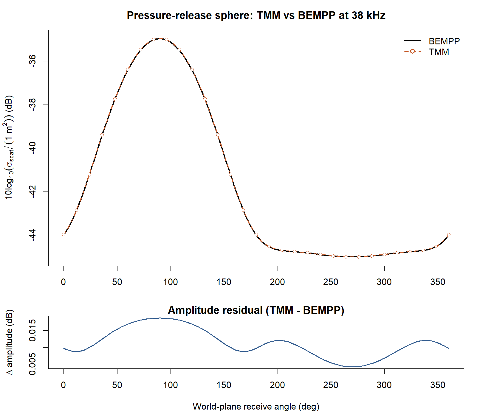
External BEM validation figures

The BEMPP pressure-release slices are a useful second validation ladder because they are independent of the in-package exact-family models. The three figures below show the broadside 38 kHz comparisons used to constrain the stored TMM angular operators.

For the sphere, the comparison is direct because the world-frame x-y slice and the body-fixed slice are identical by symmetry. For the oblate and prolate spheroids, the BEMPP world-frame slice is first converted to the same body-fixed angular convention used by tmm_scattering(). That frame conversion is what resolves the apparent nonspherical mismatch.

External BEM figures

• Sphere
• Oblate
• Prolate
• Cylinder

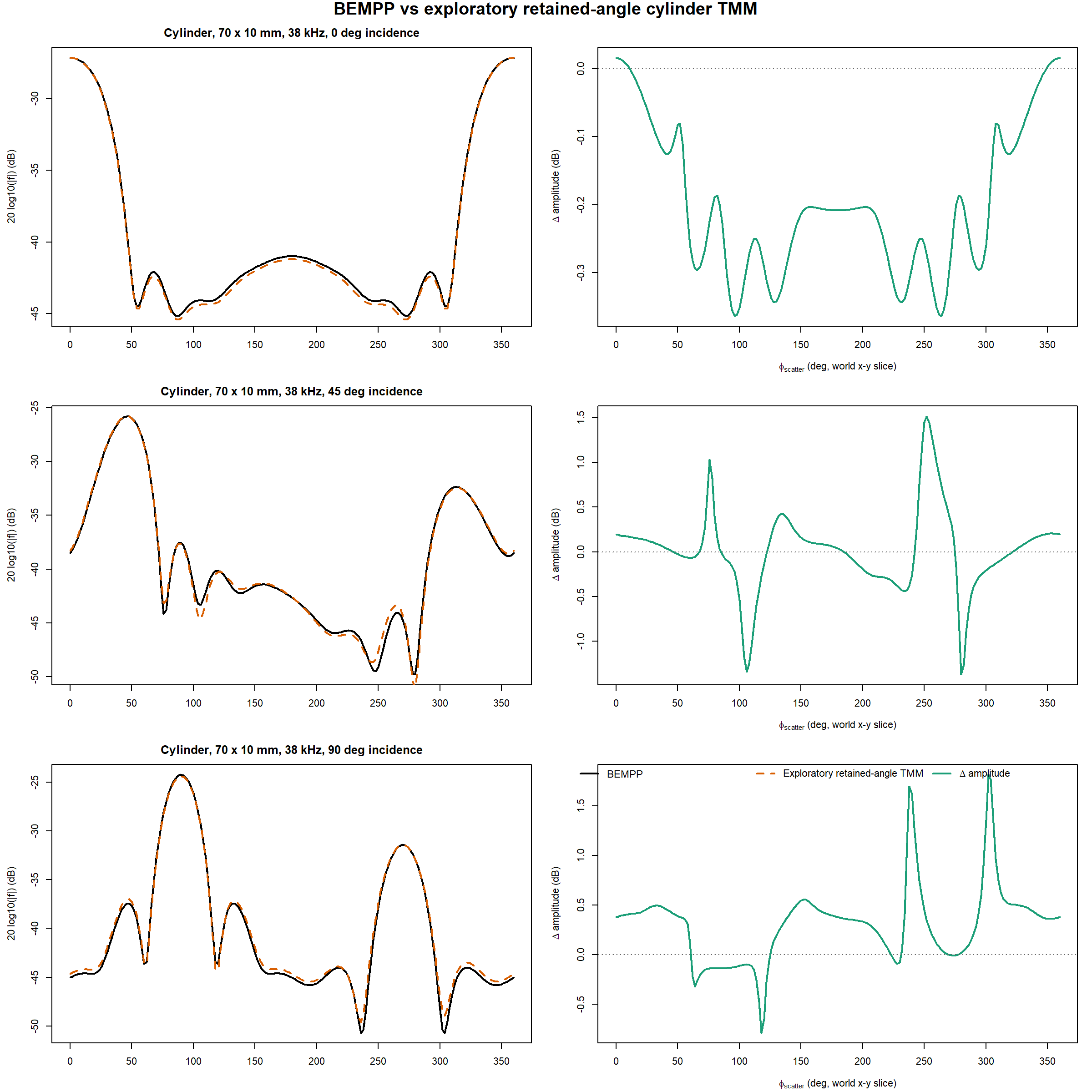
For the cylinder, the analogous full-angle figure is shown here only as a constraint on the exploratory retained-angle cylinder operator. It is not documenting a supported public cylinder workflow. The point of the figure is to show why the package refuses to provide full retained cylinder grids and bistatic summaries instead of pretending they are validated.

These figures make the external-validation story much more concrete:

1. the pressure-release sphere is externally calibrated to the BEMPP far-field solver,
2. the retained pressure-release oblate branch also agrees closely once the frame convention is matched correctly,
3. the retained pressure-release prolate branch also agrees closely once the frame convention is matched correctly,
4. the exploratory retained-angle cylinder branch does not agree externally and is therefore not part of the documented public retained-cylinder workflow, and
5. even the exact monostatic pressure-release cylinder branch is only externally close near broadside on the tested cases, so cylinder remains the least externally constrained TMM shape family and emits a warning by default when used.

At this point, no direct paper-figure reproduction is claimed here for the prolate angular response. If a future paper-grounded reproduction is added, it needs to match the original paper’s normalization, axes, and geometry conventions exactly rather than only mimicking the general visual style.

Representative spectra

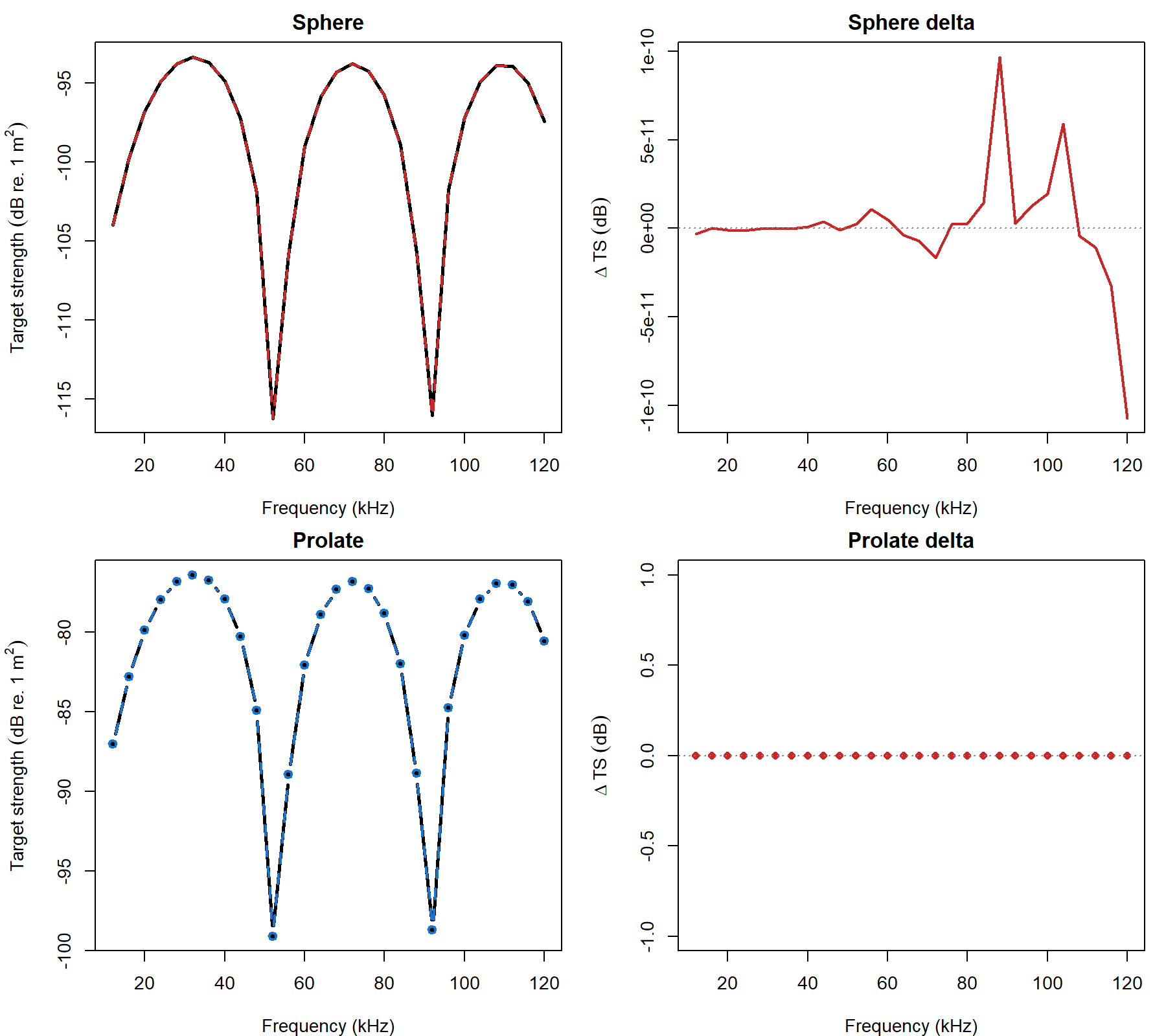
The sphere figure is the more conventional benchmark story: a T-matrix implementation agreeing with the exact spherical modal solution. The prolate figure is really a geometry-consistency story: the TMM family lands on the exact spheroidal solution rather than drifting because of a mismatched basis.

References

Ganesh, M., and Stuart C. Hawkins. 2022. “A Numerically Stable T-Matrix Method for Acoustic Scattering by Nonspherical Particles with Large Aspect Ratios and Size Parameters.” The Journal of the Acoustical Society of America 151 (3): 1978–88. https://doi.org/10.1121/10.0009679.

Waterman, P. C. 1969. “New Formulation of Acoustic Scattering.” The Journal of the Acoustical Society of America 45 (6): 1417–29. https://doi.org/10.1121/1.1911619.

———. 2009. “T -Matrix Methods in Acoustic Scattering.” The Journal of the Acoustical Society of America 125 (1): 42–51. https://doi.org/10.1121/1.3035839.