Phase-compensated distorted wave Born approximation
Source:vignettes/pcdwba/pcdwba-implementation.Rmd
pcdwba-implementation.RmdacousticTS implementation
These pages follow the phase-compensated weak-scattering literature for broadside elongated bodies and krill-style applications (Chu and Ye 1999; Chu et al. 1993).
The phase-compensated distorted wave Born approximation is available
through target_strength(..., model = "pcdwba"). The
implementation is intended for weakly scattering fluid-like bodies and
uses the same curved-cylinder bookkeeping whether the target starts as a
canonical bent cylinder or an arbitrary fluid-like profile.
This page checks the implementation against two source-level references:
- the
pcdwba_fbsroutine in thePythonpackage Echopop (Lucca and Lee (2026)), - the bent-cylinder DWBA routines in the
R-package ZooScatR (Gastauer et al. (2019)) .
PCDWBA is validated here against source-level reference
implementations rather than against a separate published benchmark
table. The ZooScatR source agrees exactly on the shared case, while the
remaining Echopop drift is attributable to that implementation’s
interpolated Bessel evaluation.
Reference case
The comparison uses a single reproducible bent-cylinder case:
- length
15 mm - radius
1 mm - taper order
10 - curvature ratio
rho_c / L = 3 - density contrast
g = 1.02 - sound-speed contrast
h = 1.02 - broadside incidence
-
12-200 kHzin2 kHzsteps -
51integration nodes in all three implementations
In acousticTS, that target is built as:
library(acousticTS)

pcdwba_object <- fls_generate(
  shape = cylinder(
    length_body = 0.015,
    radius_body = 0.001,
    taper = 10,
    radius_curvature_ratio = 3,
    n_segments = 50
  ),
  g_body = 1.02,
  h_body = 1.02,
  theta_body = pi / 2
)

pcdwba_object <- target_strength(
  object = pcdwba_object,
  frequency = seq(12e3, 200e3, by = 2e3),
  model = "pcdwba",
  sound_speed_sw = 1500,
  density_sw = 1026
)

head(extract(pcdwba_object, "model")$PCDWBA)
## frequency ka f_bs sigma_bs TS
## 1 12000 0.05026548 -6.147156e-07+7.354948e-11i 3.778753e-13 -124.2265
## 2 14000 0.05864306 -8.131273e-07+1.148885e-10i 6.611760e-13 -121.7968
## 3 16000 0.06702064 -1.027176e-06+1.682542e-10i 1.055090e-12 -119.7671
## 4 18000 0.07539822 -1.251059e-06+2.344088e-10i 1.565149e-12 -118.0544
## 5 20000 0.08377580 -1.478570e-06+3.137691e-10i 2.186169e-12 -116.6032
## 6 22000 0.09215338 -1.703221e-06+4.063858e-10i 2.900962e-12 -115.3746Validation outputs
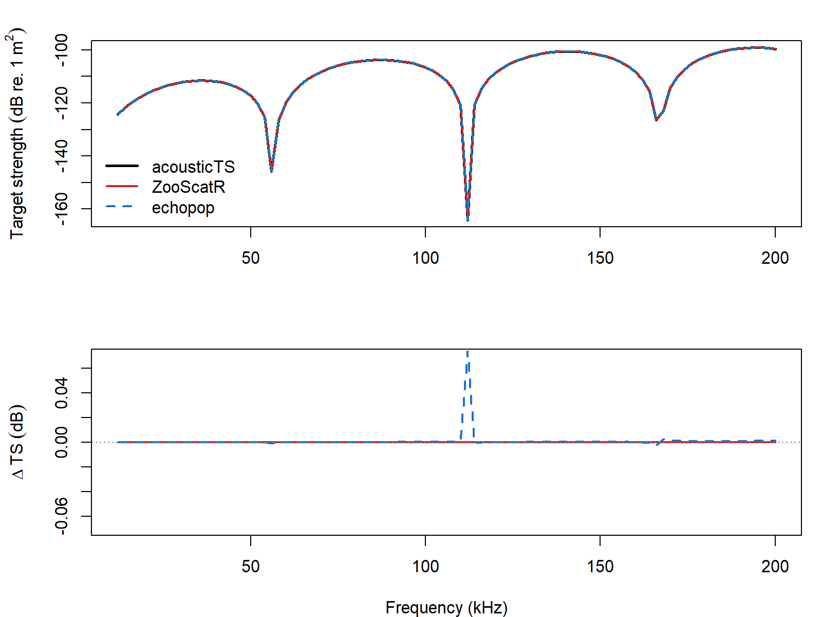
Comparison summary
| Comparison | Max abs. \Delta TS (dB) | Mean abs. \Delta TS (dB) |
|---|---|---|
| acousticTS vs echopop | 0.073947 | 0.001123 |
| acousticTS vs ZooScatR-source | 0.000000 | 0.000000 |
| echopop vs ZooScatR-source | 0.073947 | 0.001123 |
The ZooScatR and acousticTS outputs are indistinguishable on this
grid. The Echopop comparison remains close as well, but it is not at
machine precision because that implementation evaluates the cylindrical
Bessel term through interpolation rather than a direct nodewise call. On
this grid, the largest mismatch occurs near 112 kHz;
replacing the interpolated J_1(x)/x evaluation with a
direct call collapses that residual onto the acousticTS / ZooScatR
curve. So the remaining drift is numerical, not geometrical.
Closing note
This is the kind of implementation check that matters for a phase-compensated bent-cylinder solver. The comparison is not just against a benchmark curve. It is against two independently written source routines that share the same governing model. On this reference case, acousticTS reproduces the direct ZooScatR-style calculation exactly and stays very close to the Echopop implementation across the full frequency band.