Elastic-shelled sphere implementation

acousticTS implementation

Unvalidated

Overview Theory

These pages are grounded in the classical elastic-shell scattering literature for fluid-filled spherical shells (Goodman and Stern 1962; Faran 1951; Stanton 1990).

The acousticTS package uses object-based scatterers so the same implementation pattern carries across models: create a scatterer, run target_strength(), inspect the stored model output, and then compare a small set of physically important inputs. For ESSMS, the required object class is ESS, which combines a spherical shell, an optional internal fluid, and the elastic constants required for the shell solution.

ESSMS is unvalidated in the package. The benchmark family exists, but the implementation does not return finite full-grid TS values across those shell-sphere comparison sweeps, so this page documents behavior and limitations rather than benchmark-grade agreement.

Elastic-shelled sphere object generation

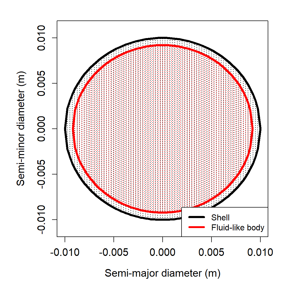
An ESS object can be created with ess_generate(). For the implementation below, the shell is described by its outer radius and thickness, while the shell material is described by density, sound speed, and elastic constants. The inner fluid can be provided using either contrasts or absolute material properties.

library(acousticTS)

sphere_shape <- sphere(radius_body = 10e-3, n_segments = 80)

shelled_sphere <- ess_generate(
  shape = sphere_shape,
  radius_shell = 10e-3,
  shell_thickness = 0.8e-3,
  density_shell = 2565,
  sound_speed_shell = 3750,
  density_fluid = 1077.3,
  sound_speed_fluid = 1575,
  E = 7.0e10,
  nu = 0.32
)

shelled_sphere

## ESS-object 
##  Elastic-shelled scatterer 
##   ID: UID 
##  Material:  
##    Shell: 
##      Density: 2565 kg m^-3
##      Sound speed: 3750 m s^-1
##      Young's modulus (E): 7e+10 Pa
##      Poisson's ratio: 0.32
##      Bulk modulus (K): 64814814814.8148 Pa
##      Shear modulus (G): 26515151515.1515 Pa  
##    Internal fluid-like body: 
##      Density: 1077.3 kg m^-3
##      Sound speed: 1575 m s^-1  
##  Shape: 
##    Shell: 
##      Radius: 0.01 m  
##      Diameter: 0.02 m  
##      Outer thickness: 8e-04 m 
##    Internal fluid-like body: 
##      Radius: 0.0092 m  
##      Diameter: 0.0184 m  
##  Propagation direction of the incident sound wave: 1.571 radians

Calculating a TS-frequency spectrum

The target_strength() wrapper initializes the ESSMS model, performs the modal calculation, and stores the results back inside the same object. As with the rest of the package, frequency is supplied in Hz.

frequency <- seq(38e3, 120e3, by = 4e3)

shelled_sphere <- target_strength(
  object = shelled_sphere,
  frequency = frequency,
  model = "essms"
)

Extracting model results

Model results can be extracted either visually or directly through extract().

Plotting results

Accessing results

essms_results <- extract(shelled_sphere, "model")$ESSMS
head(essms_results)

## $frequency
##  [1]  38000  42000  46000  50000  54000  58000  62000  66000  70000  74000
## [11]  78000  82000  86000  90000  94000  98000 102000 106000 110000 114000
## [21] 118000
## 
## $ka_shell
##  [1] 1.616199 1.786325 1.956451 2.126577 2.296703 2.466830 2.636956 2.807082
##  [9] 2.977208 3.147334 3.317461 3.487587 3.657713 3.827839 3.997965 4.168092
## [17] 4.338218 4.508344 4.678470 4.848596 5.018722
## 
## $ka_fluid
##  [1] 1.486903 1.643419 1.799935 1.956451 2.112967 2.269483 2.425999 2.582515
##  [9] 2.739032 2.895548 3.052064 3.208580 3.365096 3.521612 3.678128 3.834644
## [17] 3.991160 4.147676 4.304192 4.460709 4.617225
## 
## $f_bs
##  [1]  8.843149e-03-0.0015569837i -3.988748e-04-0.0013454280i
##  [3]  7.933887e-04-0.0020808975i  3.758589e-03-0.0025164450i
##  [5]  1.449933e-03-0.0025584566i  1.445879e-03-0.0027217379i
##  [7]  2.665126e-04-0.0029960130i  1.988643e-03-0.0033577386i
##  [9]  6.537530e-03+0.0004434971i  2.481196e-03+0.0060923410i
## [11] -2.502007e-05+0.0051816261i -1.487989e-04+0.0046774712i
## [13]  3.699388e-04+0.0044661894i  1.356868e-04+0.0043078778i
## [15]  1.445075e-03+0.0040700486i  2.348643e-03+0.0038576369i
## [17]  3.160952e-03+0.0039211202i  3.337304e-03+0.0043504980i
## [19]  3.915986e-03+0.0047782567i  2.212936e-03+0.0050012593i
## [21]  5.261250e-04+0.0046749085i
## 
## $sigma_bs
##  [1] 8.062548e-05 1.969278e-06 4.959600e-06 2.045949e-05 8.648005e-06
##  [6] 9.498424e-06 9.047123e-06 1.522911e-05 4.293599e-05 4.327295e-05
## [11] 2.684988e-05 2.190088e-05 2.008370e-05 1.857622e-05 1.865354e-05
## [16] 2.039748e-05 2.536680e-05 3.006443e-05 3.816668e-05 2.990968e-05
## [21] 2.213158e-05
## 
## $TS
##  [1] -40.93528 -57.05693 -53.04553 -46.89105 -50.63084 -50.22348 -50.43490
##  [8] -48.17325 -43.67179 -43.63783 -45.71058 -46.59538 -46.97156 -47.31043
## [15] -47.29239 -46.90423 -45.95734 -45.21947 -44.18316 -45.24188 -46.54988

The extracted data.frame contains the modeled frequency, complex backscattering amplitude f_bs, backscattering cross-section sigma_bs, and target strength TS.

Comparison workflows

Shell-thickness sensitivity

Shell thickness strongly affects the resonance structure of the ESSMS solution, so it is a natural first comparison when testing a new parameterization.

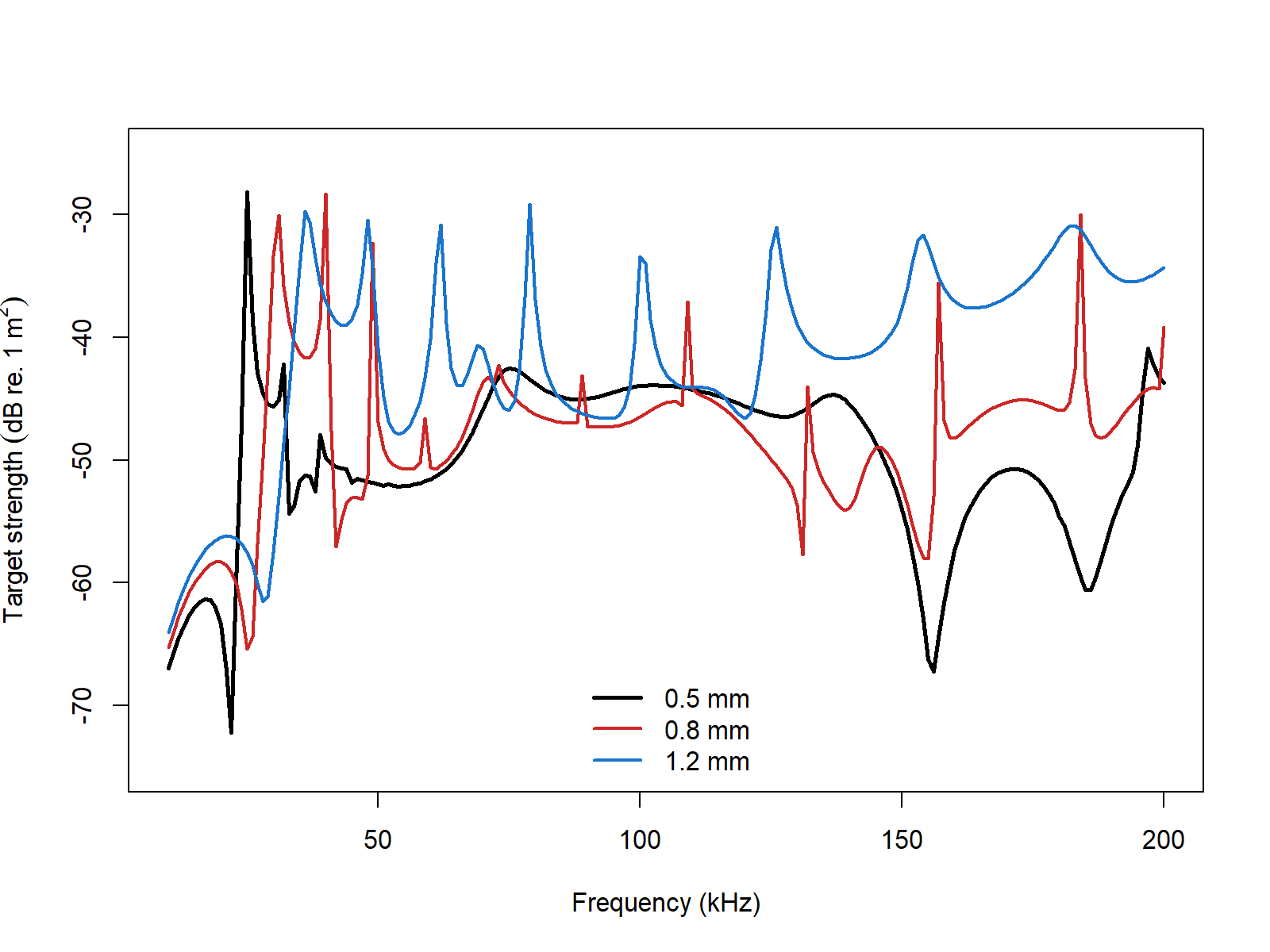
When you move from a tutorial object to a real calibration or biological shell, the next quantities to revisit are the shell elastic constants and the shell-to-fluid property contrast, because those control where the strongest modal features occur.

References

Faran, James J. 1951. “Sound Scattering by Solid Cylinders and Spheres.” The Journal of the Acoustical Society of America 23 (4): 405–18. https://doi.org/10.1121/1.1906780.

Goodman, Ralph R., and Raya Stern. 1962. “Reflection and Transmission of Sound by Elastic Spherical Shells.” The Journal of the Acoustical Society of America 34 (3): 338–44. https://doi.org/10.1121/1.1928120.

Stanton, T. K. 1990. “Sound Scattering by Spherical and Elongated Shelled Bodies.” The Journal of the Acoustical Society of America 88 (3): 1619–33. https://doi.org/10.1121/1.400321.