Your first frequency sweep

Compute rigid-sphere backscatter, check modal truncation, and save a figure and data. Install AcousticScattering and CairoMakie following Getting Started. The blocks on this page share a Julia session and execute during every documentation build.

Define and solve

using AcousticScattering
using CairoMakie: Figure, Axis, lines!, save

body = Sphere(0.01) # radius, m
boundary = Rigid()
sound_speed = 1477.4 # m/s
frequencies = collect(range(12000.0, 200000.0; length = 80)) # Hz
wavenumbers = 2pi .* frequencies ./ sound_speed
solutions = [modal(body, boundary, k) for k in wavenumbers]
strengths = target_strength.(solutions)
@assert all(isfinite, strengths)

Rigid() imposes zero total normal fluid velocity at the surface. The modal solver is a useful starting point because the sphere permits separation of variables. Each solution represents one frequency. See Choosing a solver when changing shape or material.

Check accuracy

check_wavenumber = last(wavenumbers)
coarse = modal(body, boundary, check_wavenumber; m_max = 40)
fine = modal(body, boundary, check_wavenumber; m_max = 80)
truncation_difference = abs(target_strength(fine) - target_strength(coarse))
@assert truncation_difference < 1e-6
truncation_difference

0.0

This checks modal truncation at one frequency, not the physical adequacy of a rigid-sphere model.

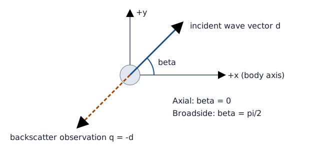
For a sphere the orientation does not change backscatter. For an axisymmetric nonspherical body, incidence and observation must be specified separately. See Conventions.

Plot and save

figure = Figure(; size = (760, 420))
axis = Axis(figure[1, 1]; xlabel = "Frequency (kHz)",
    ylabel = "Target strength (dB re 1 m²)", title = "Rigid sphere, radius 1 cm")
lines!(axis, frequencies ./ 1000, strengths; color = :navy, linewidth = 2)
save("rigid_sphere_frequency.png", figure)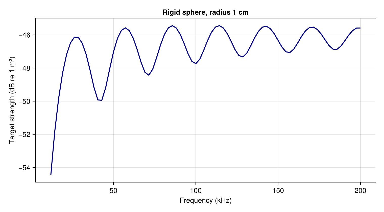

open("rigid_sphere_frequency.csv", "w") do io
    println(io, "frequency_hz,target_strength_db")
    for (frequency, strength) in zip(frequencies, strengths)
        println(io, frequency, ",", strength)
    end
end

Download the figure and CSV. In your own session, these files appear in the current working directory.

Continue with Materials and shells, Geometry and incidence, or Numerical convergence. Compilation and threading advice lives in the separate performance tutorial.