Interacting particles

Multiple scattering between two particles

Two nearby fluid particles share one coupled solve, so the pressure driving either surface already includes the field reradiated by the other. Both are exterior-facing regions (parents=[0, 0]). The oblique view keeps their facing surfaces visible, where that mutual loading is easiest to compare. The gold arrow marks the incident wave direction.

using AcousticScattering
using CairoMakie: Axis, DataAspect, Colorbar, @L_str, heatmap!, lines!, plot, save, Figure

surfaces = [
    mesh(; semiaxes=(0.012, 0.009, 0.008), center=(-0.018, 0, 0),
        resolution=0.5, qorder=4),
    mesh(; semiaxes=(0.010, 0.008, 0.007), center=(0.018, 0.006, 0),
        resolution=0.5, qorder=4)]
materials = [FluidFilled(1.4, 0.8), FluidFilled(1.8, 0.7)]
solution = bem(surfaces, materials, 300.0; parents=[0, 0],
    incidence_angle=pi / 3, incidence_azimuth=pi / 6)
fig = plot(solution; kind=:surface_field, field=:pressure_magnitude,
    colormap=:viridis, incident_arrow=true, figure=(size=(900, 580),),
    axis=(azimuth=-0.34pi, elevation=0.23pi, xlabel="x (m)",
        ylabel="y (m)", zlabel="z (m)"))
save("pair_pressure.png", fig)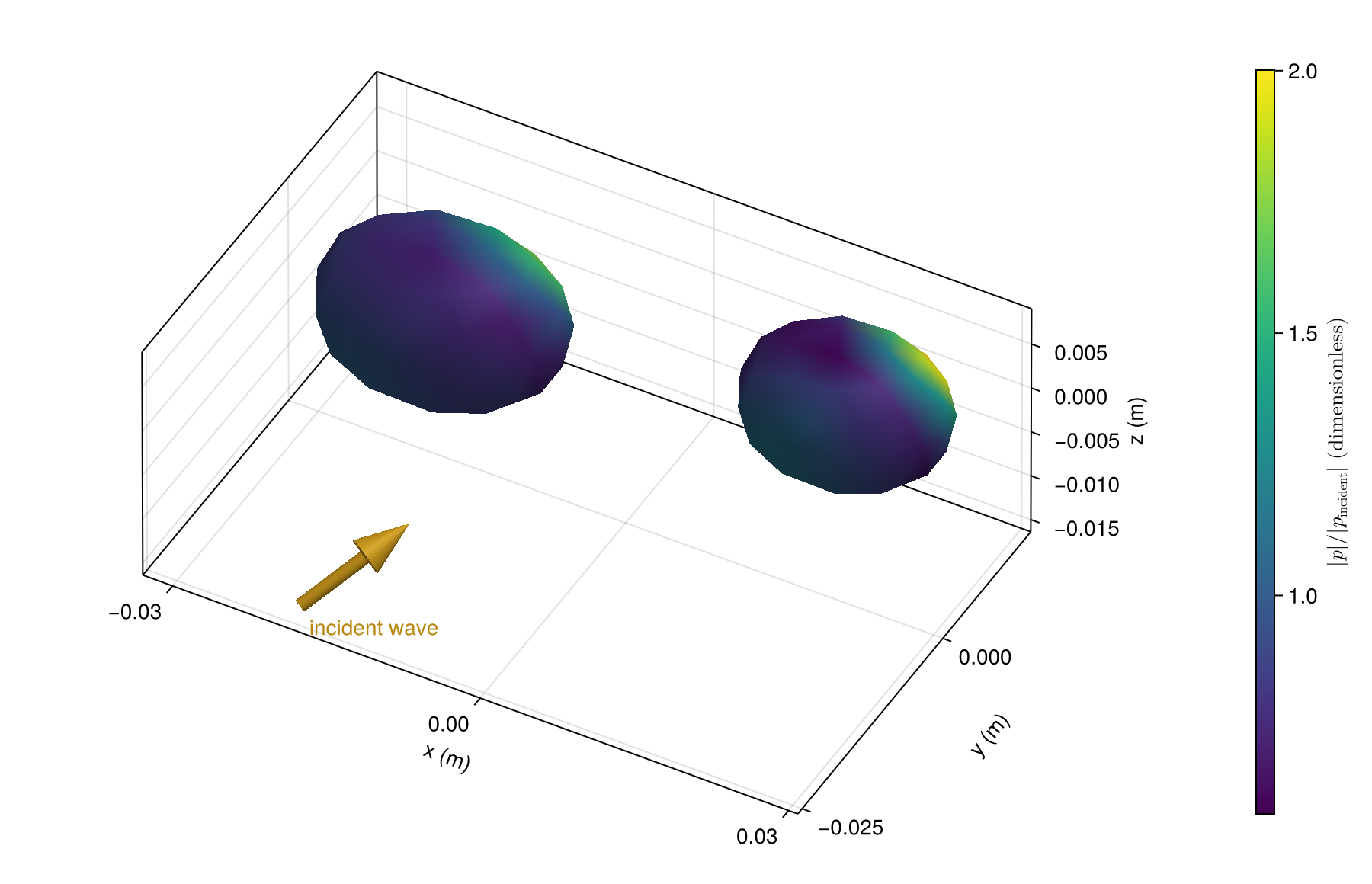

Both particles have a lower sound speed than the surrounding fluid, so each focuses the wave onto its exit side, as an isolated sphere of the same material does. A slice through z = 0 shows the field inside and around both particles.

grid = range(-0.05, 0.05; length=201)
p = pressure(solution, [(x, y, 0.0) for x in grid, y in grid])
fig = Figure(size=(900, 560))
ax = Axis(fig[1, 1]; aspect=DataAspect(), xlabel="x (mm)", ylabel="y (mm)")
hm = heatmap!(ax, 1000grid, 1000grid, real.(p)'; colormap=:balance, colorrange=(-2, 2))
theta = range(0, 2pi; length=201)
lines!(ax, 1000 .* (-0.018 .+ 0.012 .* cos.(theta)), 1000 .* (0.009 .* sin.(theta));
    color=:black, linewidth=2)
lines!(ax, 1000 .* (0.018 .+ 0.010 .* cos.(theta)), 1000 .* (0.006 .+ 0.008 .* sin.(theta));
    color=:black, linewidth=2)
Colorbar(fig[1, 2], hm; label=L"\mathrm{Re}(p / p_\mathrm{incident})~(\mathrm{dimensionless})")
save("pair_slice.png", fig)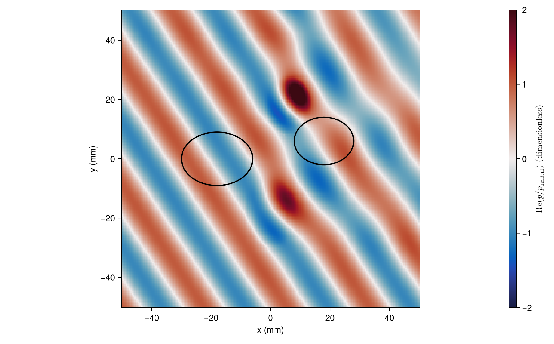

Phase across a three-body cluster

Use three differently sized particles with oblique incidence. The returned solution includes multiple scattering among all three bodies.

using AcousticScattering
using CairoMakie: Axis3, Colorbar, @L_str, plot, surface, save

surfaces = [
    mesh(; semiaxes=(0.011, 0.008, 0.007), center=(-0.020, -0.012, 0), resolution=0.5, qorder=4),
    mesh(; semiaxes=(0.010, 0.007, 0.006), center=(0.016, -0.010, 0.006), resolution=0.5, qorder=4),
    mesh(; semiaxes=(0.009, 0.007, 0.006), center=(0, 0.020, -0.005), resolution=0.5, qorder=4)]
solution = bem(surfaces, fill(FluidFilled(1.5, 0.8), 3), 400.0;
    parents=[0, 0, 0], incidence_angle=pi / 3, incidence_azimuth=pi / 4)
fig = plot(solution; kind=:surface_field, field=:pressure_phase,
    colormap=:twilight, colorrange=(-pi, pi), incident_arrow=true,
    figure=(size=(900, 580), figure_padding=(70, 20, 55, 20)),
    axis=(azimuth=-0.35pi, elevation=0.24pi, xlabel="x (m)",
        ylabel="y (m)", zlabel="z (m)"))
save("cluster_phase.png", fig)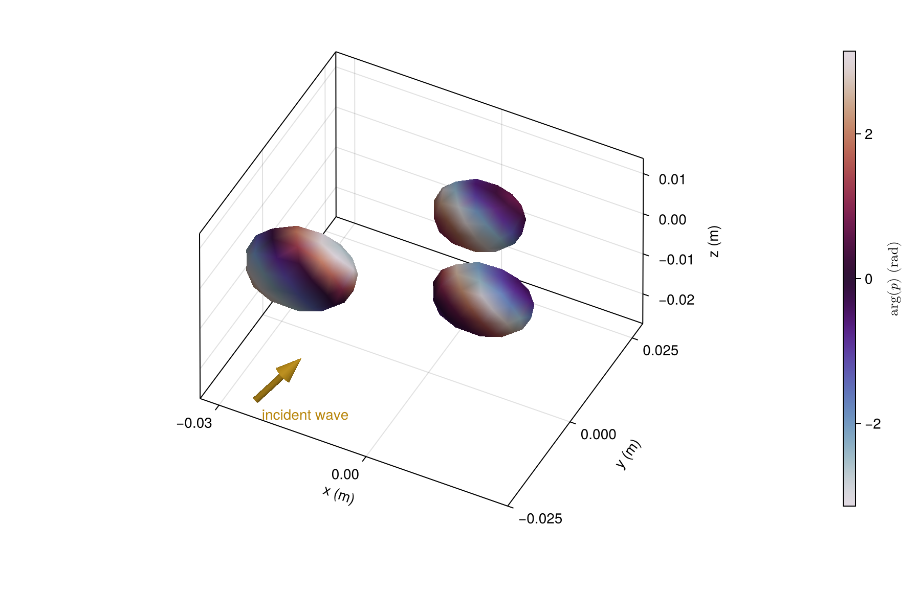

The cluster's 3D scattering pattern

Reuse that solution for every observation direction. Radius maps the upper 25 dB of response onto 0.08 to 1.0 so secondary lobes remain visible. Color is unmodified target strength. This is a directional pattern, not a physical surface, so the axes $q_x$, $q_y$, $q_z$ are direction components scaled by that radius. The small central sphere is the 0.08 radius floor, where the response is more than 25 dB below the peak. Backscatter is opposite the incident wave.

pattern = bistatic_map(solution, range(0, pi; length=91), range(0, 2pi; length=181))
peak = maximum(pattern.target_strength)
r = 0.08 .+ 0.92 .* clamp.((pattern.target_strength .- peak .+ 25) ./ 25, 0, 1)
x = r .* cos.(pattern.thetas)
y = r .* sin.(pattern.thetas) .* cos.(pattern.phis')
z = r .* sin.(pattern.thetas) .* sin.(pattern.phis')
fig = surface(x, y, z; color=pattern.target_strength, colormap=:viridis,
    figure=(size=(800, 520), figure_padding=(70, 20, 20, 20)),
    axis=(type=Axis3, aspect=:data, xlabel=L"q_x", ylabel=L"q_y", zlabel=L"q_z"))
Colorbar(fig.figure[1, 2], fig.plot; label="Target strength (dB re 1 m²)")
save("cluster_radiation.png", fig)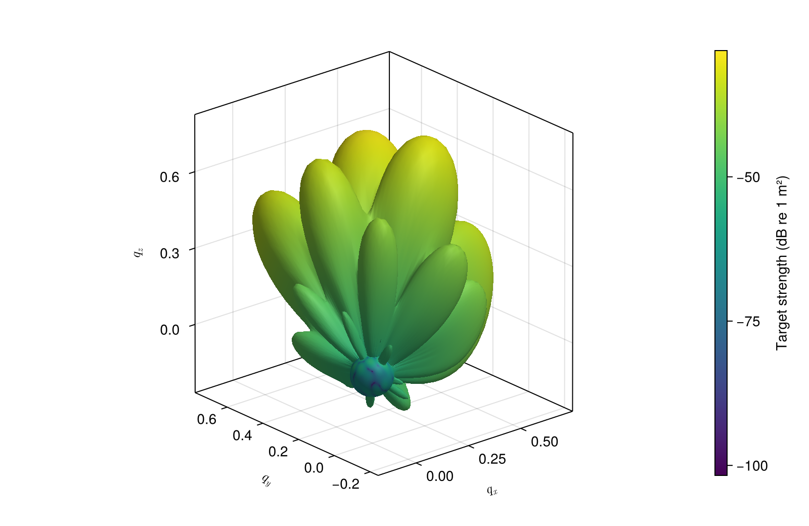

Mesh settings are compact visualization choices. Refine meshes and quadrature before using these values quantitatively.