Surface phase and directional scattering

Solve a closed rigid body with curved sides and rounded ends. Its pronounced bend lies in the xy plane and its midpoint tangent is +x. The gold arrow used below is the incident propagation direction.

using AcousticScattering
using CairoMakie: Axis3, Colorbar, Figure, Point3f, Vec3f, arrows3d!, plot, plot!,
    scale!, surface!, wireframe!, text!, save

body = Cylinder(0.005, 0.02; radius_curvature=0.012, endcap_depth=0.005)
surface_mesh = mesh(body; method=:full, resolution=0.0024, mesh_order=3, qorder=4)
beta, alpha = pi / 3, 0.4
d = Vec3f(cos(beta), sin(beta) * cos(alpha), sin(beta) * sin(alpha))
solution = bem(surface_mesh, Rigid(), 450.0;
    incidence_angle=beta, incidence_azimuth=alpha)

Phase on the surface

Color shows scattered-pressure phase. The cyclic palette joins −π and π. The higher wavenumber produces several visible phase bands instead of compressing the field into one hue.

fig = plot(solution; kind=:surface_field, field=:pressure_phase,
    colorrange=(-pi, pi), colormap=:twilight,
    figure=(size=(900, 580), figure_padding=(70, 20, 20, 20)),
    axis=(xlabel="x (m)", ylabel="y (m)", zlabel="z (m)", zlabeloffset=70,
        azimuth=-0.42pi, elevation=0.26pi))
arrows3d!(fig.axis, [Point3f(-0.022 .* d)], [0.013d]; color=:goldenrod)
Colorbar(fig.figure[1, 2]; limits=(-pi, pi), colormap=:twilight, label="Phase (rad)")
save("phase.png", fig)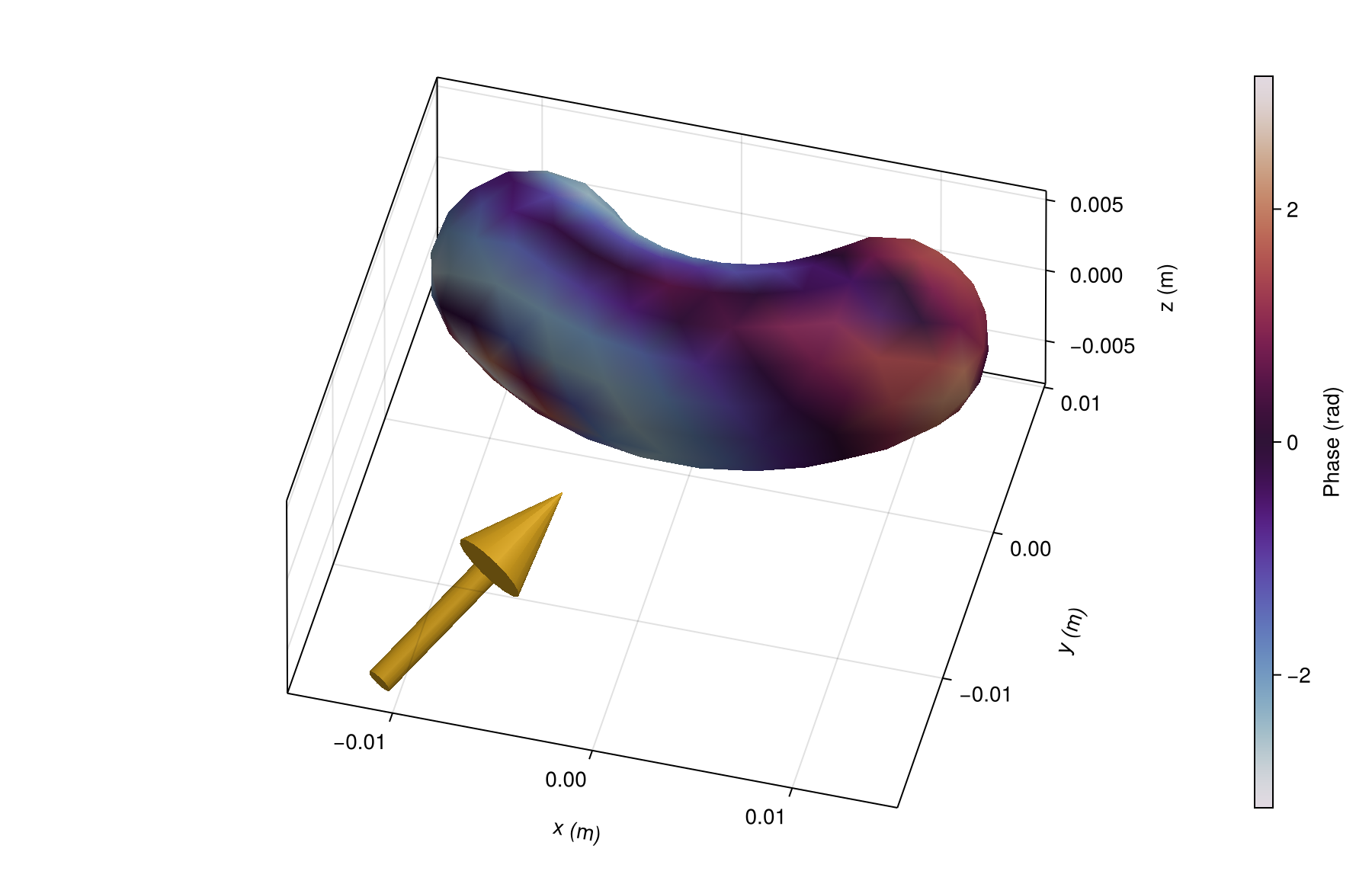

All observation directions

Keep incidence fixed and sweep observation polar angle and azimuth.

fig = plot(solution; kind=:bistatic_map,
    thetas=range(0, pi; length=181), phis=range(0, 2pi; length=361),
    colormap=:viridis, interpolate=true, figure=(size=(900, 560),),
    axis=(limits=(0, 180, 0, 360),))
Colorbar(fig.figure[1, 2], first(fig.plot.plots);
    label="Target strength (dB re 1 m²)")
save("map.png", fig)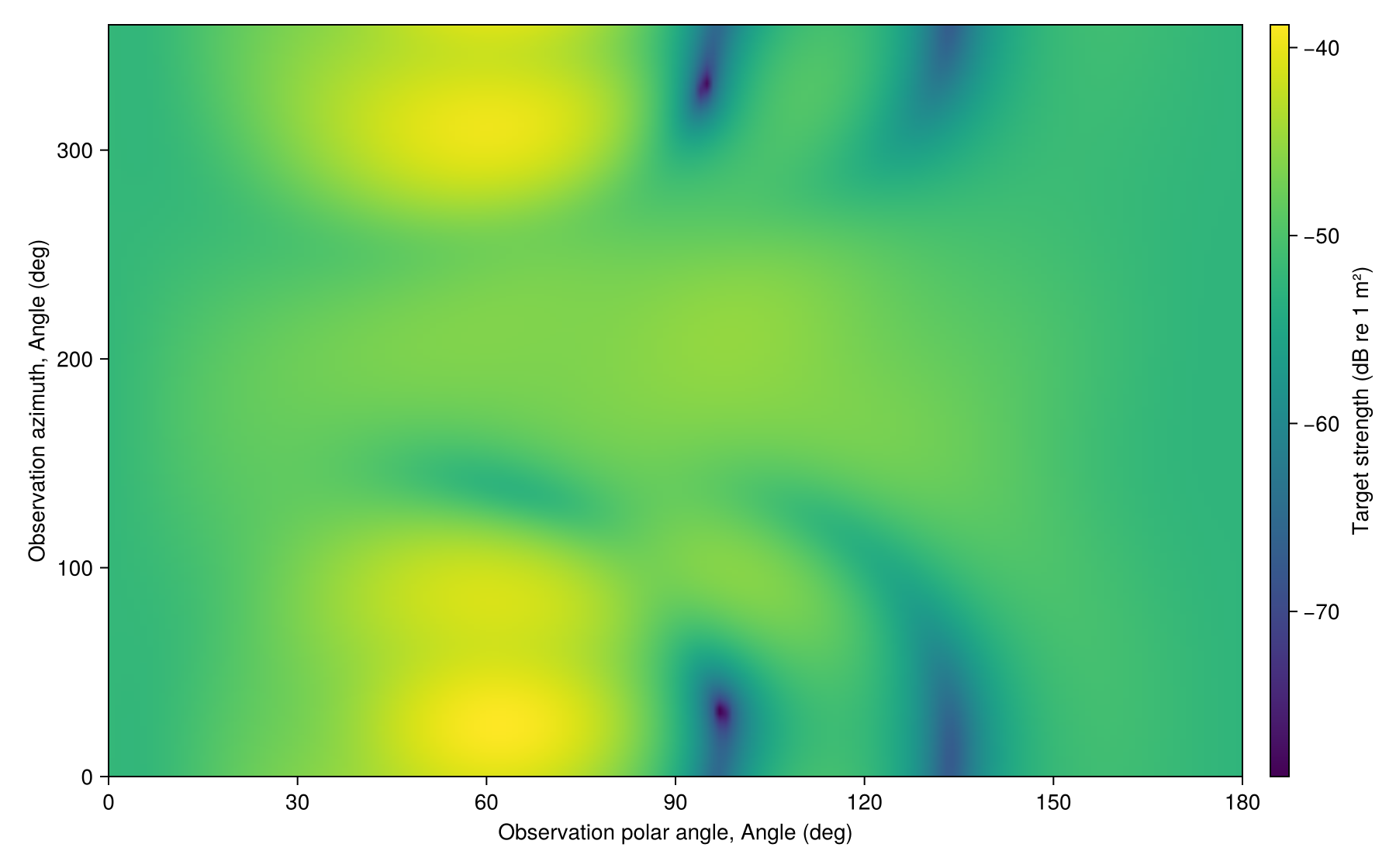

3D scattering lobes

Radius is far-field pressure amplitude divided by its maximum, while color is the unmodified target strength in dB re 1 m². The translucent pattern surrounds a scaled rendering of the bent cylinder so its orientation remains visible. The gold arrow is the incident propagation direction. The blue arrow identifies the monostatic backscatter direction, and the large downstream lobe is the forward-scattered response. Plot coordinates are dimensionless normalized-response coordinates, not physical positions.

pattern = bistatic_map(solution, range(0, pi; length=91), range(0, 2pi; length=181))
peak = maximum(pattern.target_strength)
r = 10 .^ ((pattern.target_strength .- peak) ./ 20)
x = r .* cos.(pattern.thetas)
y = r .* sin.(pattern.thetas) .* cos.(pattern.phis')
z = r .* sin.(pattern.thetas) .* sin.(pattern.phis')

fig = Figure(size=(900, 580), figure_padding=(70, 20, 20, 20))
ax = Axis3(fig[1, 1]; aspect=:data, limits=((-1, 1), (-1, 1), (-1, 1)),
    xlabel="x direction", ylabel="y direction", zlabel="z direction",
    azimuth=-0.24pi, elevation=0.16pi)
lobes = surface!(ax, x, y, z; color=pattern.target_strength, colormap=:viridis,
    alpha=0.55, transparency=true)
wireframe!(ax, x, y, z; color=(:black, 0.07), linewidth=0.35, transparency=true)

# The response coordinates are dimensionless, so enlarge the physical mesh only as a visual orientation reference. Its scale is not part of the radiation-pattern magnitude.
target = plot!(ax, surface_mesh; show_edges=true)
scale!(target, 18, 18, 18)

incident_tail = Point3f(-1.05 .* d)
arrows3d!(ax, [incident_tail], [0.28d]; color=:goldenrod,
    shaftradius=0.012, tipradius=0.04, tiplength=0.10, minshaftlength=0)
text!(ax, [incident_tail]; text=["incident"], color=:darkgoldenrod,
    fontsize=14, align=(:right, :bottom), offset=(-4, 4))
backscatter = -0.58d
arrows3d!(ax, [Point3f(0, 0, 0)], [backscatter]; color=:dodgerblue,
    shaftradius=0.012, tipradius=0.04, tiplength=0.10, minshaftlength=0)
text!(ax, [Point3f(backscatter)]; text=["backscatter"], color=:dodgerblue4,
    fontsize=14, align=(:right, :bottom), offset=(-4, 4))

Colorbar(fig[1, 2], lobes; label="Target strength (dB re 1 m²)")
save("radiation.png", fig)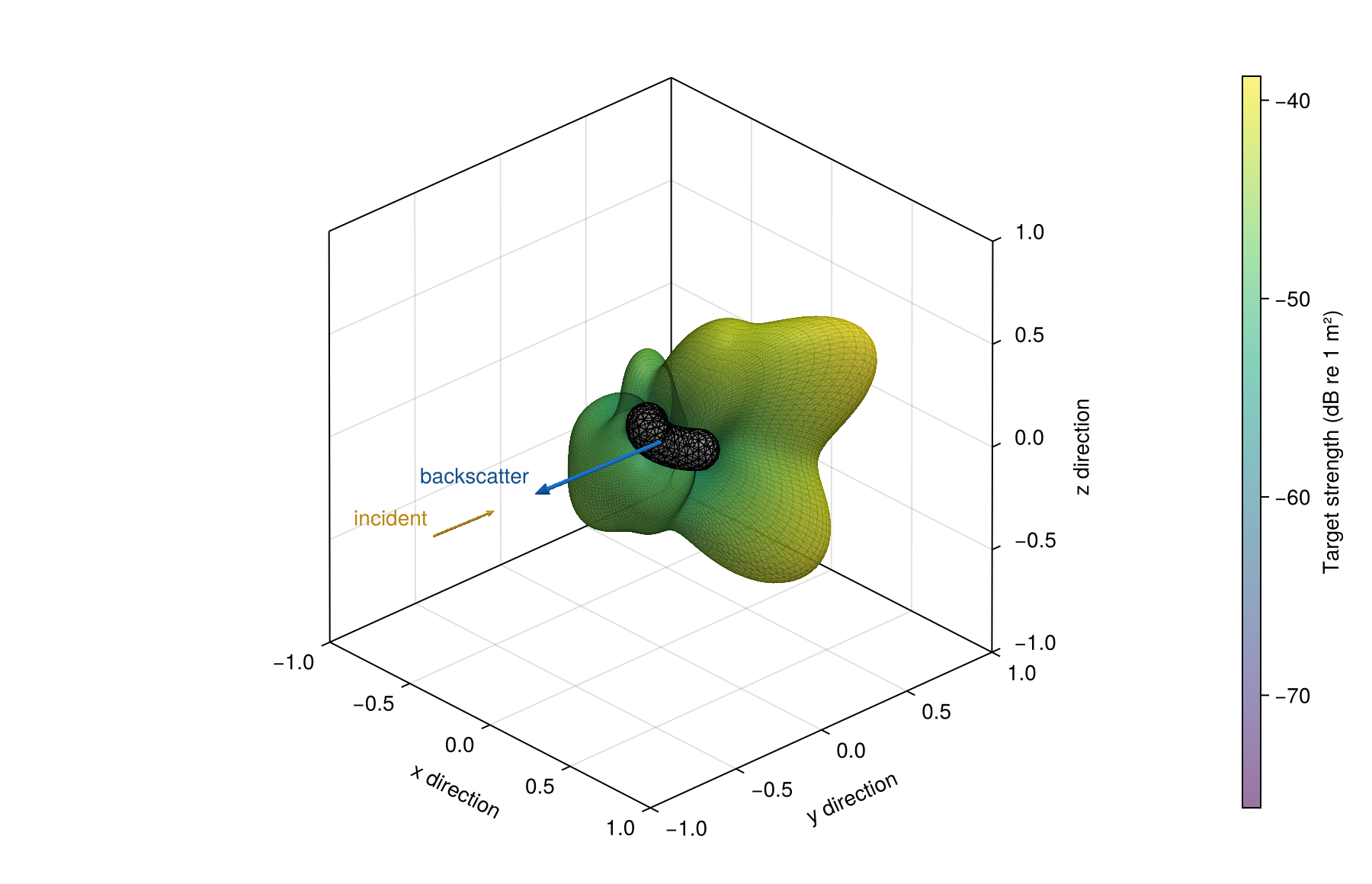

The bent-cylinder tutorial checks mesh and quadrature refinement and adds frequency and incidence sweeps.