AcousticScattering.jl
AcousticScattering.jl predicts how individual bodies scatter sound in a fluid. Construct a geometry and material configuration, solve with the following methods:
- Modal series solutions for canonical shapes
- Kirchoff physical optics and approximation
- Boundary element methods
- Method of fundamental solutions
- Finite element methods
- Fourier matching methods
Various quantities can then be extracted from these solutions such as the raw scattering amplitude, phase, and target strength (dB re. 1 m²). Compare idealized shapes, explore frequency and orientation dependence, and check numerical calculations against analytical models.
using AcousticScattering

sound_speed = 1477.4 # m/s
frequency = 38000.0 # Hz
wavenumber = 2pi * frequency / sound_speed
solution = modal(Sphere(0.01), Rigid(), wavenumber)
target_strength(solution)
-49.08829084071884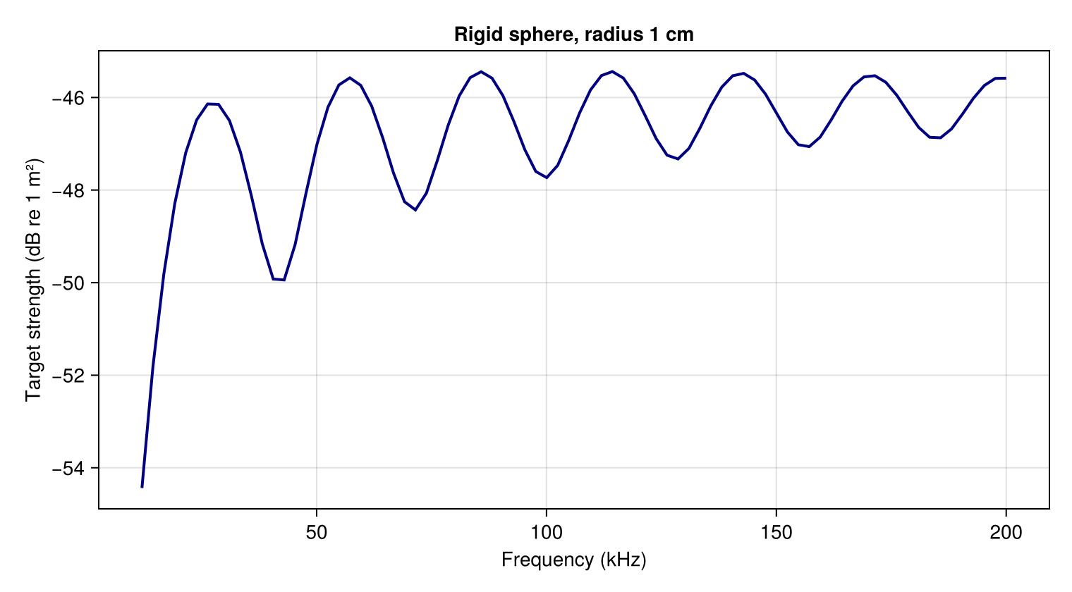
Start with Getting Started, then follow Your first frequency sweep to generate this plot and save its data. Choosing a solver lists supported combinations. The API Reference describes current calls.
Try an application
For a quick look at the package's capabilities, open the Visualization Gallery: pressure maps, 3D geometry, resonances and angular patterns, with short Julia examples.
| Question | Tutorial |
|---|---|
| How does an elastic reference target differ from a rigid sphere? | Reference-target models |
| Where is a gas bubble's scattering resonance? | Gas-bubble resonance |
| How does a coating affect scattering and internal pressure? | Coated particles |
Scope and maturity
Implemented methods include sphere/spheroid series, finite-cylinder approximations, curved-cylinder models, physical-optics surface integrals, axisymmetric and full surface BEM, radial, meridian and full 3D volume FEM, MFS, and coupled structural shells. Supported materials differ by solver and geometry. Creating a material does not guarantee support in every solver.
Full 3D volume FEM covers spheres and spheroids with elastic and shelled boundaries, and nested or disjoint fluid regions. See BEM and MFS for boundary-element formulations and irregular-frequency treatment.