Getting Started

Install into a project environment, choose whether to run the optional precompile workload, and calculate rigid-sphere target strength. The current package requires Julia 1.10 or later.

Installation

Install the package

For the current development version, install from the repository:

import Pkg
Pkg.activate("acoustic-example"; shared = false)
Pkg.add(url = "https://github.com/brandynlucca/AcousticScattering.jl")

For a version available in your configured registry, use the normal package-name form:

import Pkg
Pkg.add("AcousticScattering")

For the plotting tutorials, install CairoMakie in the same environment:

Pkg.add("CairoMakie")

CairoMakie writes static figures without a display server. Plotting is optional for numerical calculations.

Precompilation: the default

Julia normally precompiles after installation. AcousticScattering additionally runs bent-cylinder and spheroid Kirchhoff examples through PrecompileTools to cache compiled code, not scattering results. This costs extra precompile time and cache space but reduces later first-call latency. The workload does not repeat on every ordinary package load when a usable cache exists.

Opt out before the first precompile

Add this to LocalPreferences.toml beside the active environment's Project.toml before installing. Merge it into an existing file, preserving any other settings:

[AcousticScattering]
precompile_workload = false

This disables AcousticScattering's PrecompileTools workload. Normal Julia and dependency precompilation still occur. First use of the affected Kirchhoff paths may then spend time compiling. PrecompileTools already honors this preference, so no source edit or interactive installer prompt is necessary. PrecompileTools preference documentation.

Alternatively, use this Julia-only sequence. It postpones automatic precompilation and sets the preference without importing AcousticScattering:

import Pkg
Pkg.activate("acoustic-example"; shared = false)
withenv("JULIA_PKG_PRECOMPILE_AUTO" => "0") do
    Pkg.add("Preferences")
    Pkg.add(url = "https://github.com/brandynlucca/AcousticScattering.jl")
end
using Preferences: set_preferences!
set_preferences!("AcousticScattering", "precompile_workload" => false; force = true)
Pkg.precompile()
using AcousticScattering

withenv restores the previous environment-variable setting. JULIA_PKG_PRECOMPILE_AUTO=0 alone only postpones precompilation: importing the package can still trigger the workload unless the preference is set. Julia Pkg precompilation documentation.

To re-enable the workload, set the preference to true, restart Julia, and run Pkg.precompile():

using Preferences: set_preferences!
set_preferences!("AcousticScattering", "precompile_workload" => true; force = true)

Changing a compile-time preference can rebuild package and dependent caches. Set the preference in the environment you actually use.

First calculation

using AcousticScattering

radius = 0.01 # m
frequency = 38000.0 # Hz
sound_speed = 1477.4 # exterior fluid, m/s
wavenumber = 2pi * frequency / sound_speed # rad/m
solution = modal(Sphere(radius), Rigid(), wavenumber)
amplitude = scattering_amplitude(solution) # complex amplitude, m
strength = target_strength(solution) # dB re 1 m²
@assert isapprox(strength, -49.088291; atol = 1e-4)
(amplitude = amplitude, target_strength = strength)

(amplitude = -0.002974772860981237 + 0.0018672516108134965im, target_strength = -49.08829084071884)

The solver returns a ModalSolution. Use target_strength to extract its scalar result. Sphere backscatter is orientation-independent, so no incidence keyword is needed. See Conventions for normalization and Your first frequency sweep for a complete plotting workflow.

First plot

After installing CairoMakie, the following plots the same model at five frequencies:

using AcousticScattering
using CairoMakie: Figure, Axis, scatterlines!, save

frequencies = [12000.0, 38000.0, 70000.0, 120000.0, 200000.0]
strengths = [target_strength(modal(Sphere(0.01), Rigid(), 2pi * f / 1477.4))
    for f in frequencies]
figure = Figure(; size = (640, 360))
axis = Axis(figure[1, 1]; xlabel = "Frequency (kHz)",
    ylabel = "Target strength (dB re 1 m²)")
scatterlines!(axis, frequencies ./ 1000, strengths)
save("first_plot.png", figure)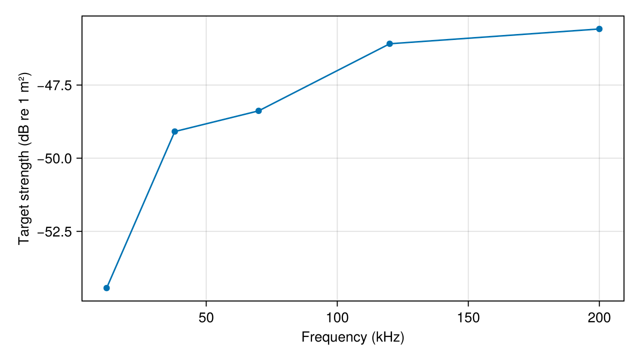

The full tutorial uses finer sampling and demonstrates saving the data and figure.

Troubleshooting

• Slow first use: distinguish downloads, dependency precompilation, and the optional workload. Compare first and second identical calls within one session to identify compilation cost.
• Artifact/Gmsh failure: retain the error and Julia/platform versions, check network or proxy access, and run Pkg.instantiate() in the active environment.
• Headless cluster: use CairoMakie and save for static figures, as in the tutorial.
• Unsupported combination: consult Choosing a solver. A material constructor does not imply support in every geometry and solver.
• Unexpected angle dependence: incidence and observation angles are distinct inputs. Review Conventions, especially for oblique axisymmetric BEM and MFS.