DWBA and SDWBA models for fluid-like scatterers

Introduction

The Distorted-Wave Born Approximation (DWBA) is a widely used theoretical framework for modeling acoustic backscatter from fluid-like organisms such as zooplankton¹ ². The DWBA treats scatterers as weakly-scattering objects with material properties that differ only slightly from the surrounding seawater. This approximation is particularly well-suited for modeling crustacean zooplankton like copepods and krill, which have body densities and sound speeds close to those of seawater.

acousticTS implementation

The acousticTS package provides four DWBA implementations for fluid-like scatterers:

DWBA: Standard DWBA for straight-bodied organisms
DWBA_curved: DWBA for organisms with curved body shapes
SDWBA: Stochastic DWBA accounting for phase variability in straight bodies
SDWBA_curved: Stochastic DWBA for curved organisms with phase variability

Both deterministic (DWBA) and stochastic (SDWBA) models are applied to objects of the FLS (Fluid-Like Scatterer) class, which can represent various zooplankton shapes from simple cylinders to complex curved forms.

# Call in package library
library(acousticTS)

## 
## Attaching package: 'acousticTS'

## The following object is masked from 'package:base':
## 
##     kappa

# Create a simple cylinder shape
cylinder_shape <- cylinder(
  length_body = 15e-3,     # 15 mm length
  radius_body = 2e-3,      # 2 mm radius
  n_segments = 50          # 50 discrete segments
)

# Create FLS object with the cylinder shape
cylinder_scatterer <- fls_generate(
  shape = cylinder_shape,
  g_body = 1.058,          # Density contrast (ρ_body/ρ_water)
  h_body = 1.058,          # Sound speed contrast (c_body/c_water)
  theta_body = pi/2        # Broadside orientation
)

# Display the object
cylinder_scatterer

## FLS-object 
##   Fluid-like scatterer 
##    ID: UID 
##  Body dimensions:
##   Length: 0.015 m (n = 51 cylinders) 
##   Mean radius: 0.002 m 
##   Max radius: 0.002 m 
##  Shape parameters:
##   Defined shape: arbitrary 
##   L/a ratio: 7.5 
##   Taper order:  
##  Material properties:
##   g: 1.058 
##   h: 1.058 
##  Body orientation (relative to transducer face/axis): 1.571 radians

Using the krill dataset

The acousticTS package includes a built-in krill dataset based on the digitized body shape from McGehee et al. (1998)³, which provides realistic morphological and material properties for Antarctic krill:

# Load the krill dataset
data(krill)

# Display basic information about the krill object
krill

## FLS-object 
##   Fluid-like scatterer 
##    ID: Antarctic Euphausia superba (McGehee et al., 1998) 
##  Body dimensions:
##   Length: 0.041 m (n = 15 cylinders) 
##   Mean radius: 0.0013 m 
##   Max radius: 0.002 m 
##  Shape parameters:
##   Defined shape: arbitrary 
##   L/a ratio: 20.1 
##   Taper order:  
##  Material properties:
##   g: 1.0357 
##   h: 1.0279 
##  Body orientation (relative to transducer face/axis): 1.571 radians

Let’s examine the krill shape:

# Plot the krill shape
plot(krill, type = "shape")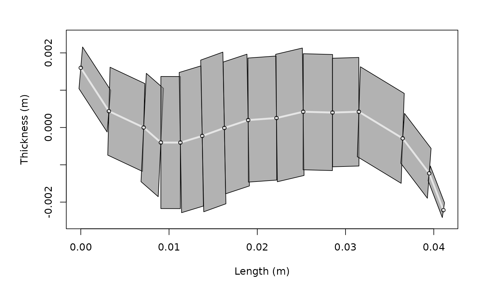

DWBA model calculations

Standard DWBA for cylindrical scatterer

The standard DWBA model assumes straight-bodied organisms and is appropriate for simple cylindrical shapes:

# Define frequency vector 
frequency <- seq(50e3, 500e3, 10e3)  # 50 kHz to 500 kHz

# Calculate TS using standard DWBA
cylinder_scatterer <- target_strength(
  object = cylinder_scatterer,
  frequency = frequency,
  model = "DWBA"
)

DWBA models for krill

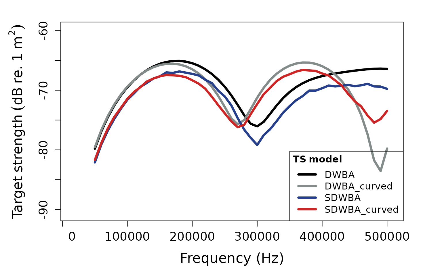
For the krill dataset, we can apply all four DWBA models to compare their performance. The curved models are more appropriate for krill due to their naturally curved body shape, while the stochastic models account for phase variability:

# Define radius-of-curvature for curved models
krill@body$radius_curvature_ratio <- 3.0

# Apply all DWBA models to krill
krill <- target_strength(
  object = krill,
  frequency = frequency,
  model = c("DWBA", "DWBA_curved", "SDWBA", "SDWBA_curved")
)

Visualizing results

Cylindrical scatterer results

# Plot TS for the cylindrical scatterer
plot(cylinder_scatterer, type = "model")

Krill model comparison

# Plot all DWBA models for krill
plot(krill, type = "model")

Model parameters and sensitivity

Extracting model results

Model results contain detailed information about the scattering calculations:

# Extract DWBA results for krill
dwba_results <- extract(krill, "model")$DWBA
head(dwba_results)

##   frequency        ka         f_bs     sigma_bs        TS
## 1     5e+04 0.3104522 0.0001023018 1.046565e-08 -79.80234
## 2     6e+04 0.3725426 0.0001431207 2.048355e-08 -76.88595
## 3     7e+04 0.4346331 0.0001882204 3.542691e-08 -74.50667
## 4     8e+04 0.4967235 0.0002361991 5.578999e-08 -72.53444
## 5     9e+04 0.5588139 0.0002855616 8.154545e-08 -70.88600
## 6     1e+05 0.6209044 0.0003347646 1.120673e-07 -69.50521

# Extract curved DWBA results
dwba_curved_results <- extract(krill, "model")$DWBA_curved
head(dwba_curved_results)

##   frequency        ka         f_bs     sigma_bs        TS
## 1     5e+04 0.3104522 0.0001050585 1.103729e-08 -79.57138
## 2     6e+04 0.3725426 0.0001466901 2.151797e-08 -76.67199
## 3     7e+04 0.4346331 0.0001924496 3.703684e-08 -74.31366
## 4     8e+04 0.4967235 0.0002408010 5.798511e-08 -72.36683
## 5     9e+04 0.5588139 0.0002901058 8.416137e-08 -70.74887
## 6     1e+05 0.6209044 0.0003386728 1.146992e-07 -69.40439

The DWBA results include: - frequency: transmit frequency (Hz) - k_sw: acoustic wavenumber for seawater - f_bs: complex backscattering amplitude - sigma_bs: backscattering cross-section (m²) - TS: target strength (dB re. 1 m²)

Material property effects

Let’s explore how different material properties affect the target strength:

# Create scatterers with different density contrasts
high_contrast <- fls_generate(
  shape = cylinder_shape,
  g_body = 1.10,    # Higher density contrast
  h_body = 1.058,
  theta_body = pi/2
)

low_contrast <- fls_generate(
  shape = cylinder_shape,
  g_body = 1.02,    # Lower density contrast  
  h_body = 1.058,
  theta_body = pi/2
)

# Calculate TS for both
high_contrast <- target_strength(high_contrast, frequency, "DWBA")
low_contrast <- target_strength(low_contrast, frequency, "DWBA")

# Extract results
ts_high <- extract(high_contrast, "model")$DWBA
ts_low <- extract(low_contrast, "model")$DWBA
ts_original <- extract(cylinder_scatterer, "model")$DWBA

# Plot comparison
plot(x = ts_original$frequency * 1e-3, 
     y = ts_original$TS, 
     type = 'l',
     lty = 1, 
     lwd = 2.5,
     xlab = "Frequency (kHz)",
     ylab = expression(Target~strength~(dB~re.~1~m^2)),
     cex.lab = 1.3, 
     cex.axis = 1.2)

lines(x = ts_high$frequency * 1e-3,
      y = ts_high$TS,
      col = 'darkgoldenrod3',
      lty = 1,
      lwd = 2.5)

lines(x = ts_low$frequency * 1e-3,
      y = ts_low$TS,
      col = 'cornflowerblue',
      lty = 1,
      lwd = 2.5)

legend("bottomright",
       c("g = 1.058 (original)", "g = 1.10 (high)", "g = 1.02 (low)"),
       lty = c(1, 1, 1),
       lwd = c(2.5, 2.5, 2.5),
       col = c('black', 'darkgoldenrod3', 'cornflowerblue'),
       cex = 1.0)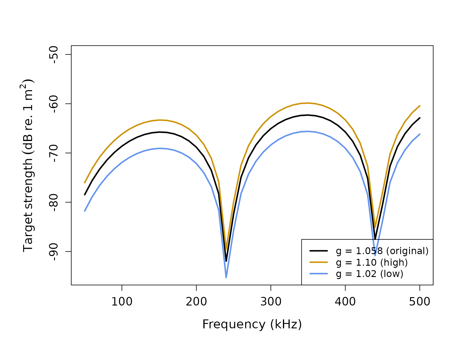

Orientation effects

The DWBA is highly sensitive to the orientation of the scatterer relative to the incident sound wave. Let’s examine this effect:

# Create scatterers at different orientations
broadside <- fls_generate(
  shape = cylinder_shape,
  g_body = 1.058, h_body = 1.058,
  theta_body = pi/2    # 90° - broadside
)

oblique <- fls_generate(
  shape = cylinder_shape,
  g_body = 1.058, h_body = 1.058,
  theta_body = pi/4    # 45° - oblique
)

end_on <- fls_generate(
  shape = cylinder_shape,
  g_body = 1.058, h_body = 1.058,
  theta_body = 0       # 0° - end-on
)

# Calculate TS for all orientations
broadside <- target_strength(broadside, frequency, "DWBA")
oblique <- target_strength(oblique, frequency, "DWBA")
end_on <- target_strength(end_on, frequency, "DWBA")

# Extract results
ts_broadside <- extract(broadside, "model")$DWBA
ts_oblique <- extract(oblique, "model")$DWBA
ts_end_on <- extract(end_on, "model")$DWBA

# Plot orientation comparison
plot(x = ts_broadside$frequency * 1e-3, 
     y = ts_broadside$TS, 
     type = 'l',
     lty = 1, 
     lwd = 2.5,
     xlab = "Frequency (kHz)",
     ylab = expression(Target~strength~(dB~re.~1~m^2)),
     cex.lab = 1.3, 
     cex.axis = 1.2)

lines(x = ts_oblique$frequency * 1e-3,
      y = ts_oblique$TS,
      col = 'darkgoldenrod2',
      lty = 1,
      lwd = 2.5)

lines(x = ts_end_on$frequency * 1e-3,
      y = ts_end_on$TS,
      col = 'firebrick3',
      lty = 1,
      lwd = 2.5)

legend("bottomright",
       c("Broadside (90°)", "Oblique (45°)", "End-on (0°)"),
       lty = c(1, 1, 1),
       lwd = c(2.5, 2.5, 2.5),
       col = c('black', 'darkgoldenrod2', 'firebrick3'),
       cex = 1.0)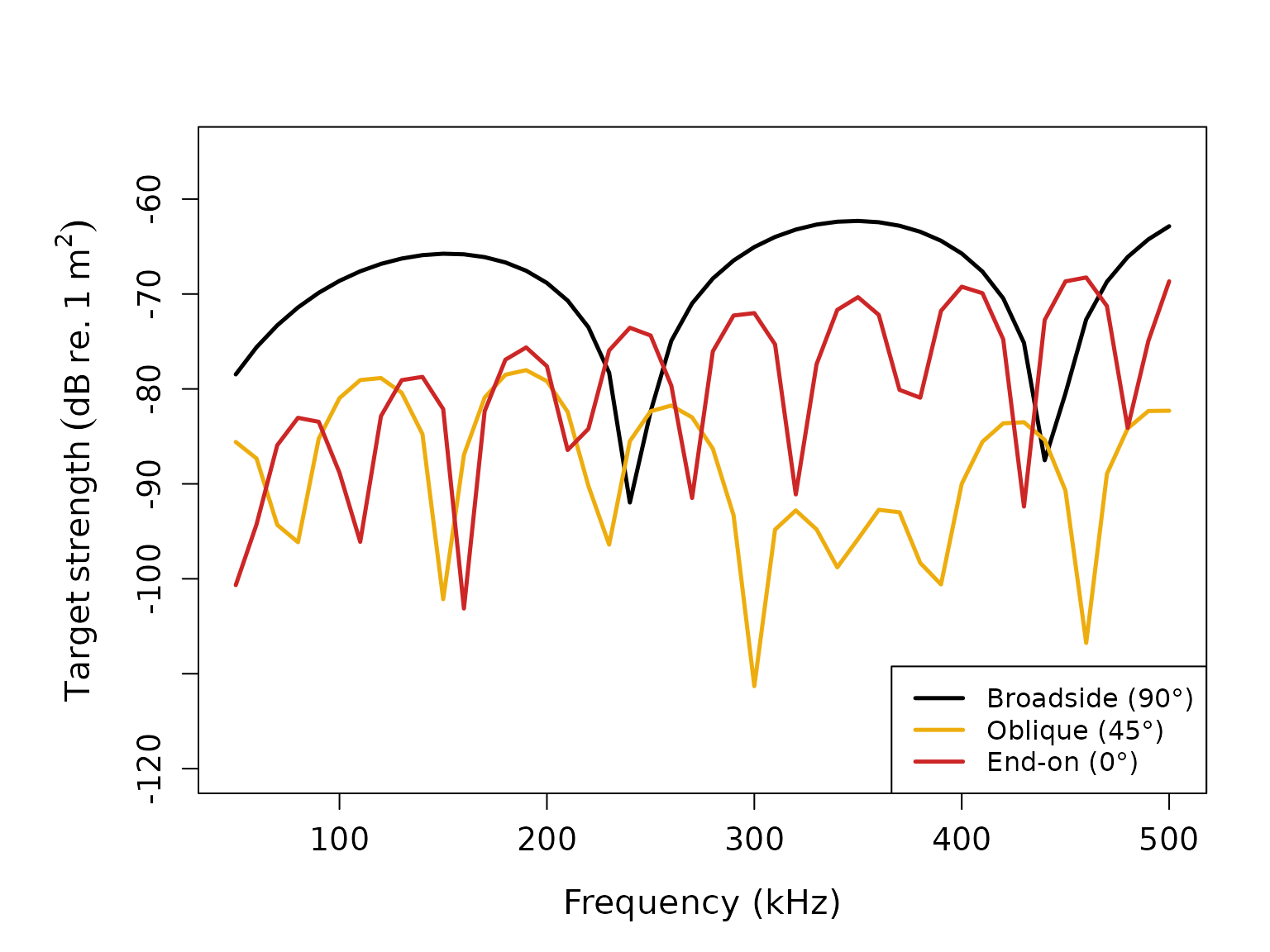

Creating custom shapes

The acousticTS package allows for creating custom shapes beyond simple cylinders. Here’s an example using a polynomial-deformed cylinder based on Smith et al. (2013)⁴:

# Create a polynomial deformation vector (example coefficients)
poly_coeffs <- c(0.83, 0.36, -2.10, -1.20, 0.63, 0.82, 0.64)  # Smith et al. (2013)

# Create a polynomial-deformed cylinder
poly_shape <- polynomial_cylinder(
  length_body = 15e-3,
  radius_body = 2e-3,
  n_segments = 50,
  polynomial = poly_coeffs
)

# Create FLS object with polynomial shape
poly_scatterer <- fls_generate(
  shape = poly_shape,
  g_body = 1.058,
  h_body = 1.058,
  radius_curvature_ratio = 3.0,
  theta_body = pi/2
)

# Calculate TS
poly_scatterer <- target_strength(
  object = poly_scatterer,
  frequency = frequency,
  model = "DWBA_curved"  # Use curved DWBA for deformed shapes
)

# Plot the polynomial-deformed shape
plot(poly_scatterer, type = "shape")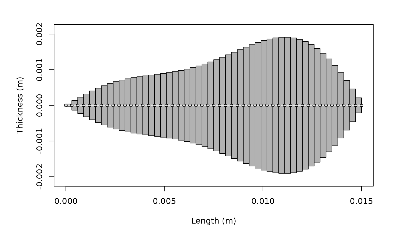

# Compare with regular cylinder
ts_poly <- extract(poly_scatterer, "model")$DWBA_curved
ts_cylinder <- extract(cylinder_scatterer, "model")$DWBA

plot(x = ts_cylinder$frequency * 1e-3, 
     y = ts_cylinder$TS, 
     type = 'l',
     lty = 1, 
     lwd = 2.5,
     col = 'cornflowerblue',
     xlab = "Frequency (kHz)",
     ylab = expression(Target~strength~(dB~re.~1~m^2)),
     cex.lab = 1.3, 
     cex.axis = 1.2)

lines(x = ts_poly$frequency * 1e-3,
      y = ts_poly$TS,
      col = 'darkseagreen4',
      lty = 2,
      lwd = 2.5)

legend("bottomright",
       c("Regular cylinder", "Polynomial-deformed cylinder"),
       lty = c(1, 2),
       lwd = c(2.5, 2.5),
       col = c('cornflowerblue', 'darkseagreen4'),
       cex = 1.0)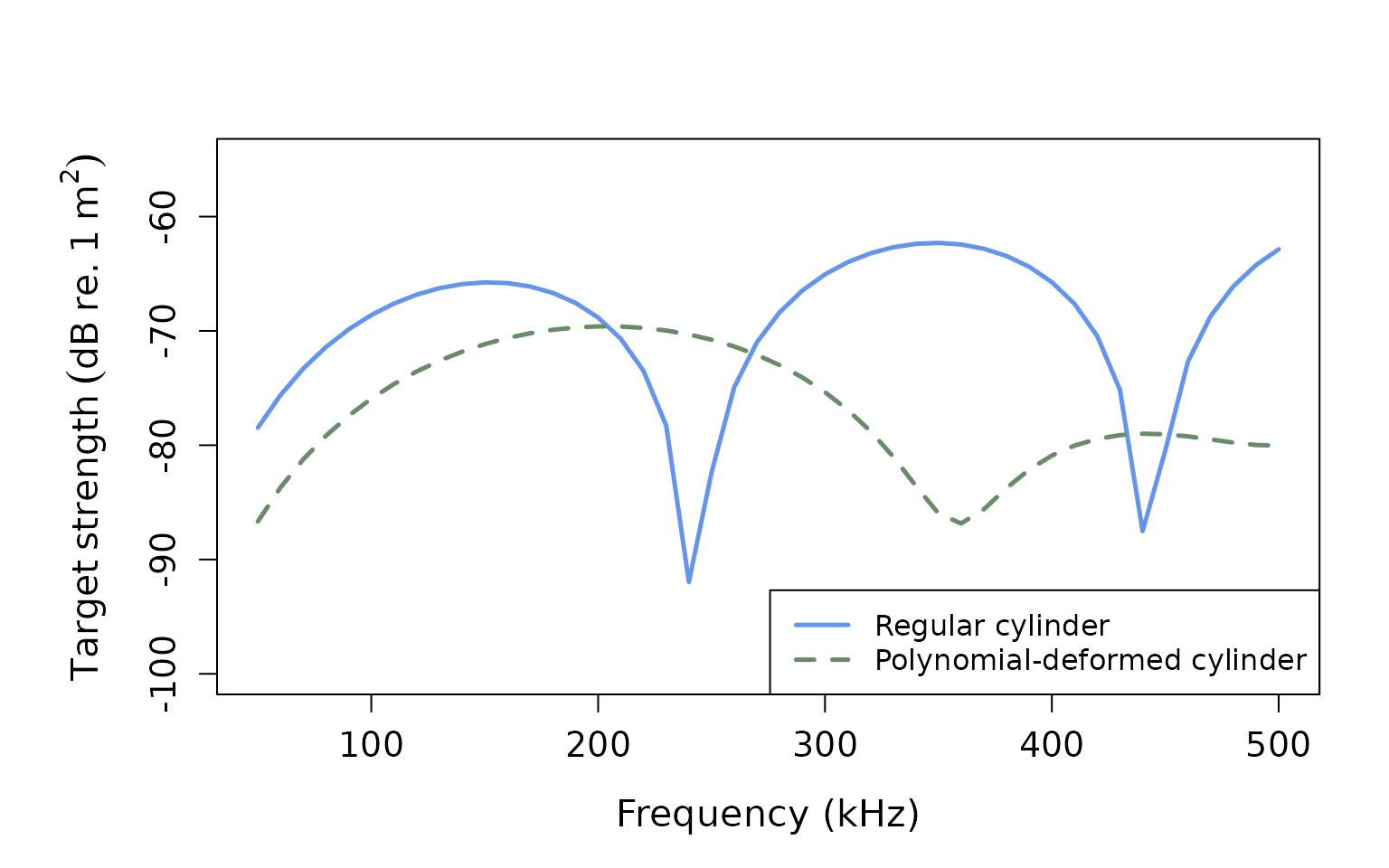

Model applications and validity

When to use DWBA vs. DWBA_curved

DWBA: Best for straight-bodied organisms or when computational speed is important
DWBA_curved: More accurate for naturally curved organisms like krill, but computationally more intensive

Biological applications

The DWBA models are particularly well-suited for:

Copepods: Small crustacean zooplankton with approximately cylindrical bodies
Krill: Larger crustaceans with naturally curved body shapes
Chaetognaths: Arrow worms with elongated, transparent bodies
Small fish larvae: When swim bladders are not yet developed

Model limitations

The DWBA has several important limitations:

Weak scattering assumption: Valid only when material contrasts are small (g, h ≈ 1)
Single scattering: Does not account for multiple scattering within the organism
Shape assumptions: Assumes cylindrical segments; complex 3D shapes may require other approaches

Future development

Future enhancements may include:

Stochastic DWBA implementations (SDWBA)
Integration with empirical orientation distributions
Automated parameter estimation from morphological data
Support for temperature and pressure-dependent material properties

Brandyn Lucca (https://orcid.org/0000-0003-3145-2969)