Target strength for a calibration sphere

Introduction

Echosounders are often calibrated using standard targets that comprise strong scatterers with target strengths (TS, dB re. 1 m²) that are relatively straightforward to model and predict¹. Typically, this comprises a tungsten carbide (chemical formula: WC) sphere, but elastic spheres consisting of other materials (e.g. aluminum, Al) can also be used².

acousticTS implementation

The acousticTS package adapts the series of equations described in the literature³ that provide a solution of wave equations based on the classical theory of elasticity. The object-based approach in acousticTS makes this relatively straightforward by minimizing the amount of manual coding end-users must write.

Calibration sphere object generation

First, a calibration sphere object has to be created. This is represented by the CAL object class that contains slots for metadata, model_parameters, model results, body for sphere dimensions and material properties, and shape_parameters for shape-specific metadata. This object can be created using the cal_generate(...) function that has two required arguments: material and diameter. The default diameter is 38.1 mm, or 38.1e^-3 m. The diameter input is intended to be in meters.The material argument comprises five default options that automatically include their respective longitudinal and transversal sound speeds (m s^-1) and material density (kg m^-3):

Material	Argument value	Longitudinal sound speed (c_l)	Transversal sound speed (c_t)	Density ( $\rho$ )
Tungsten carbide	“WC”	6853	4171	8360
Aluminum	“Al”	6260	3080	2070
Stainless steel	“steel”	5980	3297	7970
Brass	“brass”	4372	2100	8360
Copper	“Cu”	4760	2288.5	8947

Alternatively, you can define your own material properties by assigning values to sound_speed_longitudinal, sound_speed_transversal, and density_sphere within cal_generate(...) such as:

cal_generate(..., density_sphere = 1026)

When using the default arguments:

# Call in package library
library(acousticTS)

## 
## Attaching package: 'acousticTS'

## The following object is masked from 'package:base':
## 
##     kappa

# Create calibration sphere object
cal_sphere <- cal_generate()
# this is equivalent to: cal_sphere <- cal_generate(material = "WC", diameter = 38.1e-3)

Calculating a TS-frequency spectrum for the calibration sphere

With the calibration sphere object generated, TS can be calculated via the target_strength(...) function, which is a wrapper function that generally allows for multiple models to be applied to a single scatterer when needed. In this case, there are three required arguments to calculate TS: object, frequency, and model. The object argument simply refers to the CAL object that we created before (i.e. cal_sphere). Frequency (via frequency) can be a vector of values (Hz). Model is a string input that refers to the model end-users would like to use, which would be model = "calibration" in this case. This will update the current CAL object when assigned to the same variable, or can be used to generate a copy of the original CAL object that now includes model parameter and results as a built-in field.

# Define frequency vector 
frequency <- seq(1e3, 600e3, 1e3)
# Calculate TS; update original CAL object
cal_sphere <- target_strength(object = cal_sphere,
                              frequency = frequency, 
                              model = "calibration")
# Calculate TS; store in a new CAL object
cal_sphere_copy <- target_strength(object = cal_sphere,
                                   frequency = frequency, 
                                   model = "calibration")

Extracting model results

Model results can be extracted either just visually, or can be directly accessed using the extract(...) function.

Plotting results

This approach uses the plot(...) generic function with additional arguments for toggling the plot output. The additional arguments to include here are:

type = "shape" or type = "model"
nudge_y = 1.05 (default)
nudge_x = 1.01 (default)
x_units = "frequency" or x_units = "k_sw" or x_units = "k_l" or x_units = "k_t"

Setting type = "model" will parse the model results (i.e. TS). The two nudge_ arguments allow the end-user to nudge to x- and y-axes as they see fit. The x_units argument defaults to x_units = "frequency", but setting it to equal "k_sw", "k_l", or "k_t" will set TS to be a function of the wavenumber of seawater, longitudinal axis of sphere, and transversal axis of sphere, respectively multiplied by the sphere’s radius.

# Plot TS as a function of frequency (kHz)
plot(cal_sphere, type = "model", ylim = c(-70, -30))

# Plot TS as a function of k[sw]*radius, or k[sw]*a
plot(cal_sphere, type = "model", x_units = "k_sw", ylim = c(-70, -30))

# Plot TS as a function of k[l]*radius, or k[sw]*a
plot(cal_sphere, type = "model", x_units = "k_l", ylim = c(-70, -30))

# Plot TS as a function of k[t]*radius, or k[sw]*a
plot(cal_sphere, type = "model", x_units = "k_t", ylim = c(-70, -30))

# Nudge the x-axis more
plot(cal_sphere, type = "model", ylim = c(-70, -30))

# Nudge the y-axis more
plot(cal_sphere, type = "model", ylim = c(-70, -30))

Accessing results

The model results can also be directly accessed via extract(...) which has the two arguments object and feature. In this case, object refers to our CAL object, cal_sphere, and we can set feature = "model" to extract our model results.

# Extract model results
model_results <- extract( cal_sphere, "model" )$calibration
# Peek at the output from extract(...)
head( model_results )

##   frequency         ka         f_bs     sigma_bs        TS
## 1      1000 0.07979645 9.444014e-05 8.918941e-09 -80.49687
## 2      2000 0.15959291 3.738998e-04 1.398010e-07 -68.54490
## 3      3000 0.23938936 8.269858e-04 6.839055e-07 -61.65004
## 4      4000 0.31918581 1.435280e-03 2.060028e-06 -56.86127
## 5      5000 0.39898227 2.174015e-03 4.726341e-06 -53.25475
## 6      6000 0.47877872 3.012785e-03 9.076873e-06 -50.42064

Here we get seven columns formatted as a data.frame object:

frequency: transmit frequency (Hz)
k_sw: acoustic wavenumber for seawater/ambient fluid
k_l: longitudinal axis acoustic wavenumber of sphere
k_t: transversal axis acoustic wavenumber of sphere
f_bs: the complex form function output
sigma_bs: the acoustic cross-section for an elastic sphere (m²) where: $\sigma_{bs} = \pi a^2 ~|f_{bs}|^2$
TS: the target strength (dB re. 1 m²) for an elastic sphere where: $TS = 10log_{10}(\frac{\sigma_{bs}}{4 \pi})$

Material property and sphere shape comparisons

This implementation also allows for comparisons among different model parameters and diameters suited for specific calibration experiments.

Comparing different diameters

# Generate models for calibration spheres
# 20 mm diameter sphere
sphere_20 <- cal_generate(diameter = 20e-3)
sphere_20 <- target_strength(object = sphere_20,
                             frequency = frequency,
                             model = "calibration")
ts_mods_20 <- extract(sphere_20, "model")$calibration
# 30 mm diameter sphere
sphere_30 <- cal_generate(diameter = 30e-3)
sphere_30 <- target_strength(object = sphere_30,
                             frequency = frequency,
                             model = "calibration")
ts_mods_30 <- extract(sphere_30, "model")$calibration
# 40 mm diameter sphere
sphere_40 <- cal_generate(diameter = 40e-3)
sphere_40 <- target_strength(object = sphere_40,
                             frequency = frequency,
                             model = "calibration")
ts_mods_40 <- extract(sphere_40, "model")$calibration
# Plot the three and compare
plot(x = ts_mods_20$frequency*1e-3, 
     y = ts_mods_20$TS, 
     type = 'l',
     lty = 1, 
     lwd = 2.5,
     xlab = "Frequency (kHz)",
     ylab = expression(Target~strength~(dB~re.~1~m^2)),
     cex.lab = 1.3, 
     cex.axis = 1.2,
     ylim = c(-70, -30))
lines(x = ts_mods_30$frequency*1e-3,
      y = ts_mods_30$TS,
      col = 'red',
      lty = 1,
      lwd = 2.5)
lines(x = ts_mods_40$frequency*1e-3,
      y = ts_mods_40$TS,
      col = 'blue',
      lty = 1,
      lwd = 2.5)
legend("bottomright",
       c("20 mm","30 mm", "40 mm"),
       lty=c(1, 1, 1),
       lwd=c(2.5, 2.5, 2.5),
       col=c('black', 'red', 'blue'),
       cex=1.1)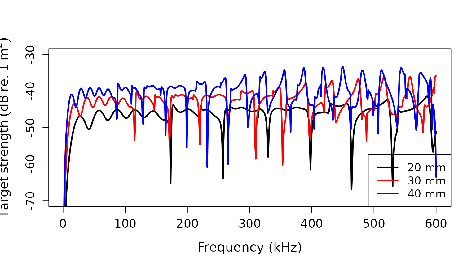

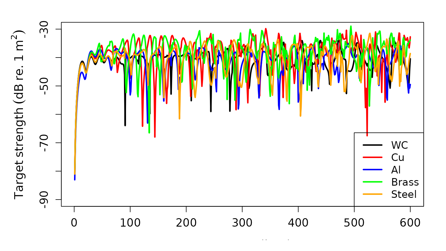
Comparing different materials

# tungsten carbide
ts_mods_WC <- extract(cal_sphere, "model")$calibration
# copper sphere
sphere_copper <- cal_generate(material = "Cu")
sphere_copper <- target_strength(object = sphere_copper,
                                 frequency = frequency,
                                 model = "calibration")
ts_mods_Cu <- extract(sphere_copper, "model")$calibration
# aluminum sphere
sphere_aluminum <- cal_generate(material = "Al")
sphere_aluminum <- target_strength(object = sphere_aluminum,
                                   frequency = frequency,
                                   model = "calibration")
ts_mods_Al <- extract(sphere_aluminum, "model")$calibration
# brass sphere
sphere_brass <- cal_generate(material = "brass")
sphere_brass <- target_strength(object = sphere_brass,
                                frequency = frequency,
                                model = "calibration")
ts_mods_brass <- extract(sphere_brass, "model")$calibration
# stainless steel sphere
sphere_steel <- cal_generate(material = "steel")
sphere_steel <- target_strength(object = sphere_steel,
                                frequency = frequency,
                                model = "calibration")
ts_mods_steel<- extract(sphere_steel, "model")$calibration
# Plot each and compare
par(ask = F,
    oma = c(1, 1, 1, 0),
    mar = c(3, 4.5, 1, 2))
plot(x = ts_mods_WC$frequency*1e-3, 
     y = ts_mods_WC$TS, 
     type = 'l',
     lty = 1, 
     lwd = 2.5,
     xlab = "Frequency (kHz)",
     ylab = expression(Target~strength~(dB~re.~1~m^2)),
     cex.lab = 1.3, 
     cex.axis = 1.2,
     ylim = c(-90, -30))
lines(x = ts_mods_Cu$frequency*1e-3,
      y = ts_mods_Cu$TS,
      col = 'red',
      lty = 1,
      lwd = 2.5)
lines(x = ts_mods_Al$frequency*1e-3,
      y = ts_mods_Al$TS,
      col = 'blue',
      lty = 1,
      lwd = 2.5)
lines(x = ts_mods_brass$frequency*1e-3,
      y = ts_mods_brass$TS,
      col = 'green',
      lty = 1,
      lwd = 2.5)
lines(x = ts_mods_steel$frequency*1e-3,
      y = ts_mods_steel$TS,
      col = 'orange',
      lty = 1,
      lwd = 2.5)
legend("bottomright",
       c("WC","Cu", "Al", "Brass", "Steel"),
       lty=c(1, 1, 1, 1, 1),
       lwd=c(2.5, 2.5, 2.5, 2.5, 2.5),
       col=c('black', 'red', 'blue', 'green', 'orange'),
       cex=1.1)

Future development

Stay tuned for new methods enabling backscatter simulations for calibration spheres of different materials, sizes, etc., from a single function rather than repeating the same dataflow.

Brandyn Lucca (https://orcid.org/0000-0003-3145-2969)